## Diagram: Saddle Point vs. Minimum ### Overview The image presents two 3D diagrams illustrating the concepts of a saddle point and a minimum in a two-dimensional space defined by parameters alpha (α) and beta (β). Each diagram shows a surface representing a function's value over the α-β plane, along with curves indicating the Hessian directions. ### Components/Axes * **Axes:** The diagrams have two axes labeled α and β, representing the two parameters. The vertical axis implicitly represents the function's value. * **Surface:** A blue-shaded surface represents the function's value over the α-β plane. The surface has a grid on it. * **Hessian Directions:** Two dark blue curves on each surface indicate the Hessian directions. These are labeled as κ₊^(α,β) and κ₋^(α,β). * **Critical Point:** A dark blue dot marks the critical point (where the gradient is zero) on each surface. * **Titles:** The diagrams are titled "(a) Saddle" and "(b) Minimum". * **Conditions:** Above each diagram, conditions are stated regarding the curvatures: * Saddle: κ₊^(α,β) * κ₋^(α,β) < 0 * Minimum: κ₊^(α,β) > 0, κ₋^(α,β) > 0 * **Footer:** "Hessian directions η, δ" ### Detailed Analysis **Diagram (a): Saddle** * The surface has a saddle shape, with a minimum along one direction and a maximum along another. * The critical point is located at the saddle point. * The curve labeled κ₊^(α,β) rises away from the saddle point. * The curve labeled κ₋^(α,β) descends away from the saddle point. * The condition κ₊^(α,β) * κ₋^(α,β) < 0 indicates that the product of the curvatures along the two Hessian directions is negative, which is characteristic of a saddle point. **Diagram (b): Minimum** * The surface has a bowl shape, indicating a minimum. * The critical point is located at the minimum. * Both curves labeled κ₊^(α,β) and κ₋^(α,β) rise away from the minimum. * The condition κ₊^(α,β) > 0, κ₋^(α,β) > 0 indicates that the curvatures along both Hessian directions are positive, which is characteristic of a minimum. ### Key Observations * The diagrams visually represent the difference between a saddle point and a minimum based on the shape of the surface and the curvatures along the Hessian directions. * The conditions stated above each diagram mathematically define the nature of the critical point. ### Interpretation The image illustrates how the Hessian matrix (specifically, the curvatures along the Hessian directions) can be used to classify critical points of a function. A saddle point occurs when the curvatures have opposite signs (one positive, one negative), while a minimum occurs when both curvatures are positive. This is a fundamental concept in optimization and calculus, used to find and characterize extrema of functions. The Hessian directions η, δ are the eigenvectors of the Hessian matrix, indicating the directions of maximum and minimum curvature.

\n ## Diagram: Saddle Point and Minimum Illustration ### Overview The image presents two 3D diagrams illustrating the concepts of a saddle point (a) and a minimum (b) in a two-dimensional space defined by axes α and β. Both diagrams depict a curved surface, with annotations indicating curvature values. The diagrams are side-by-side for comparison. ### Components/Axes * **Axes:** Both diagrams share the same axes labeled α (x-axis) and β (y-axis). * **Curvature Labels:** Each diagram features two curvature labels: κ^α,β₊ and κ^α,β_-. These labels are positioned on the curved surface to indicate the direction of curvature. * **Conditions:** Each diagram includes a mathematical condition relating the curvature values: * **(a) Saddle:** κ^α,β₊ κ^α,β_- < 0 * **(b) Minimum:** κ^α,β₊ > 0, κ^α,β_- > 0 * **Hessian Directions:** Below the second diagram, the text "Hessian directions η, δ" is present. ### Detailed Analysis / Content Details **Diagram (a) - Saddle Point:** * The surface resembles a saddle, with upward curvature along the α-axis and downward curvature along the β-axis. * The label κ^α,β₊ is positioned on the upward-curving portion of the surface, near the α-axis. * The label κ^α,β_- is positioned on the downward-curving portion of the surface, near the β-axis. * The condition κ^α,β₊ κ^α,β_- < 0 indicates that the product of the curvatures is negative, which is characteristic of a saddle point. **Diagram (b) - Minimum:** * The surface curves upwards in both the α and β directions, forming a bowl-like shape. * The label κ^α,β₊ is positioned on the upward-curving portion of the surface, near the α-axis. * The label κ^α,β_- is positioned on the upward-curving portion of the surface, near the β-axis. * The condition κ^α,β₊ > 0, κ^α,β_- > 0 indicates that both curvatures are positive, which is characteristic of a minimum. ### Key Observations * The diagrams visually demonstrate the difference between a saddle point and a minimum. * The curvature labels and conditions provide a mathematical description of these concepts. * The Hessian directions are mentioned, suggesting a connection to the Hessian matrix used in optimization problems. * The diagrams are simplified representations, focusing on the curvature rather than precise numerical values. ### Interpretation The diagrams illustrate fundamental concepts in multivariable calculus and optimization. The saddle point represents a critical point where the function has zero gradient, but it is not a local minimum or maximum. The minimum represents a point where the function reaches its lowest value in a local region. The curvature values (κ^α,β₊ and κ^α,β_-) quantify the rate of change of the function along the α and β axes, respectively. The conditions provided relate these curvature values to the type of critical point. The mention of Hessian directions suggests that these diagrams are relevant to the second derivative test, which uses the Hessian matrix to determine the nature of critical points. The diagrams are useful for visualizing these abstract concepts and understanding their geometric interpretation.

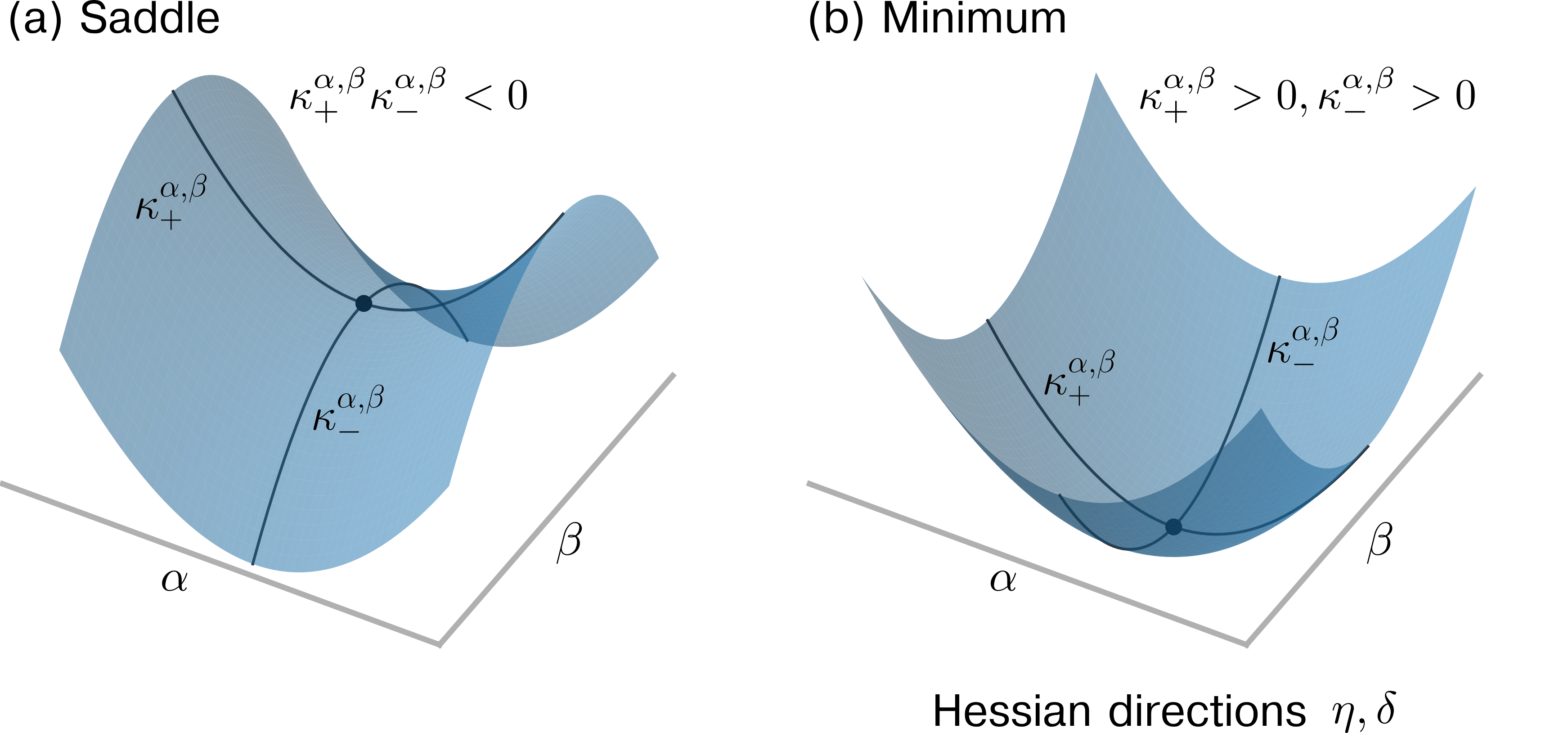
## Mathematical Diagram: Saddle Point vs. Minimum on a 2D Surface ### Overview The image displays two side-by-side 3D surface plots illustrating the geometric interpretation of critical points on a two-variable function. The left diagram (a) depicts a saddle point, while the right diagram (b) depicts a local minimum. Both plots are rendered as blue, semi-transparent surfaces with a visible grid pattern, set against a white background. The diagrams are labeled with mathematical notation describing the principal curvatures at the central critical point. ### Components/Axes **Spatial Layout:** - The image is divided into two distinct panels. - **Panel (a) - Left:** Titled "(a) Saddle" in the top-left corner. - **Panel (b) Right:** Titled "(b) Minimum" in the top-right corner. - A caption at the bottom center reads: "Hessian directions η, δ". **Axes (Common to both plots):** - Each plot features a 3D coordinate system with two horizontal axes. - The axis extending from the bottom-left towards the center is labeled **α** (alpha). - The axis extending from the bottom-right towards the center is labeled **β** (beta). - These axes define the domain plane over which the surface is plotted. The vertical axis (function value) is not explicitly labeled. **Surface Elements:** - **Central Point:** A black dot marks the critical point (where the gradient is zero) at the center of each surface. - **Curves:** Two dark blue curves are drawn on each surface, intersecting at the central point. These represent the paths of principal curvature. - **Curvature Labels:** - In both plots, one curve is labeled **κ₊^{α,β}** (kappa-plus, with superscripts α,β). - The other curve is labeled **κ₋^{α,β}** (kappa-minus, with superscripts α,β). **Mathematical Annotations:** - **Panel (a) Saddle:** An equation is placed near the top of the surface: **κ₊^{α,β} κ₋^{α,β} < 0**. - **Panel (b) Minimum:** An equation is placed near the top of the surface: **κ₊^{α,β} > 0, κ₋^{α,β} > 0**. ### Detailed Analysis **Diagram (a) - Saddle Point:** - **Surface Shape:** The surface curves upward along one principal direction and downward along the other, creating a classic saddle or hyperbolic paraboloid shape. The central point is a minimax point. - **Curvature Relationship:** The annotation **κ₊^{α,β} κ₋^{α,β} < 0** indicates that the two principal curvatures have opposite signs. This is the defining mathematical condition for a saddle point in two dimensions. - **Curve Behavior:** The curve labeled **κ₊^{α,β}** appears to follow a path where the surface curves upward (convex) from the central point. The curve labeled **κ₋^{α,β}** follows a path where the surface curves downward (concave) from the central point. **Diagram (b) - Minimum:** - **Surface Shape:** The surface curves upward in all directions from the central point, forming a bowl or valley shape. The central point is the lowest point in its local neighborhood. - **Curvature Relationship:** The annotation **κ₊^{α,β} > 0, κ₋^{α,β} > 0** indicates that both principal curvatures are positive. This is the defining mathematical condition for a local minimum in two dimensions. - **Curve Behavior:** Both curves, **κ₊^{α,β}** and **κ₋^{α,β}**, follow paths where the surface curves upward (convex) away from the central point. **Bottom Caption:** - The text **"Hessian directions η, δ"** suggests that the two principal curvature directions (κ₊ and κ₋) correspond to the eigenvectors (η, δ) of the Hessian matrix evaluated at the critical point. The Hessian matrix contains the second partial derivatives of the function. ### Key Observations 1. **Visual Contrast:** The diagrams provide a clear visual contrast between a saddle point (indefinite Hessian) and a minimum (positive definite Hessian). 2. **Geometric Interpretation:** The curves on the surfaces are not arbitrary; they represent the directions of maximum and minimum curvature (principal directions) at the critical point. 3. **Mathematical Notation:** The use of superscripts (α,β) on the curvature symbols (κ) explicitly ties these geometric properties to the coordinate system defined by the α and β axes. 4. **Color and Style:** The consistent use of blue for the surface, black for the critical point and curves, and gray for the axes creates a clean, technical aesthetic focused on conveying mathematical concepts. ### Interpretation These diagrams are fundamental visualizations in multivariable calculus, optimization theory, and differential geometry. They illustrate how the second derivative test (via the Hessian matrix) classifies critical points. - **What the data suggests:** The diagrams demonstrate that the sign of the product of the principal curvatures (or equivalently, the determinant of the Hessian) determines the type of critical point. A negative product indicates a saddle point, while two positive curvatures indicate a minimum. (By extension, two negative curvatures would indicate a maximum). - **How elements relate:** The axes (α, β) define the input space. The surface height represents the function value. The curves (κ₊, κ₋) show the paths of steepest ascent/descent in curvature, which are the eigenvectors of the Hessian. The equations summarize the curvature conditions that define the point's nature. - **Notable patterns/anomalies:** The key pattern is the direct link between algebraic conditions (signs of κ) and geometric shape. There are no anomalies; the diagrams are canonical representations. The "Hessian directions" caption explicitly connects the geometric principal directions to the algebraic eigenvectors of the second-derivative matrix, unifying the visual and analytical perspectives. In essence, this image serves as a pedagogical tool to bridge the gap between the abstract algebra of second derivatives and the tangible geometry of surfaces, showing why a saddle point is neither a max nor a min, and how a minimum "holds water" from all directions.

## 3D Function Visualization: Saddle Point vs. Minimum ### Overview The image contains two 3D surface plots comparing critical points in a multivariable function. Plot (a) shows a saddle point configuration, while plot (b) illustrates a minimum point. Both plots use α and β as independent variables on orthogonal axes, with implicit third-axis values representing function output. ### Components/Axes - **Axes Labels**: - Horizontal axes: α (x-axis), β (y-axis) - Vertical axis: Implicit function value (z-axis) - **Mathematical Labels**: - κ+α,β and κ−α,β annotations on both plots - Hessian directions η, δ labeled at bottom of plot (b) - **Color Coding**: - Light blue shading for surface areas - Dark blue lines for critical point contours - Black dots marking critical points ### Detailed Analysis #### Plot (a) Saddle Point - **Surface Structure**: - Hyperbolic paraboloid shape with opposing curvature - Central black dot at intersection of κ+ and κ− contours - **Mathematical Conditions**: - κ+α,β < 0 and κ−α,β < 0 (both negative definite) - Critical point occurs where surface crosses itself - **Spatial Features**: - Left side shows upward curvature (α-direction) - Right side shows downward curvature (β-direction) #### Plot (b) Minimum - **Surface Structure**: - Parabolic bowl shape with single global minimum - Central black dot at lowest point - **Mathematical Conditions**: - κ+α,β > 0 and κ−α,β > 0 (both positive definite) - Hessian directions η, δ indicate gradient paths - **Spatial Features**: - All directions curve upward from central minimum - Contour lines form concentric ellipses around minimum ### Key Observations 1. **Curvature Sign Relationship**: - Saddle point (a) shows mixed curvature signs (one positive, one negative) - Minimum (b) shows uniform positive curvature 2. **Hessian Directionality**: - Only present in minimum plot (b) - Arrows point toward minimum along principal axes 3. **Critical Point Identification**: - Saddle point marked by intersecting surface - Minimum marked by lowest surface point 4. **Symmetry**: - Both plots show bilateral symmetry about α=0 and β=0 ### Interpretation The visualization demonstrates fundamental concepts in multivariable calculus: 1. **Saddle Point Significance**: - Represents unstable equilibrium where function increases in one direction and decreases in another - Mathematical manifestation of competing gradients 2. **Minimum Characteristics**: - Stable equilibrium point with positive definite Hessian - Indicates local/global optimization target 3. **Hessian Geometry**: - Directions η, δ in plot (b) show paths of steepest descent - Elliptical contour patterns confirm quadratic approximation validity 4. **Practical Implications**: - Saddle points often represent transition states in physical systems - Minima correspond to equilibrium states in optimization problems - Curvature analysis provides insight into function behavior near critical points The plots effectively demonstrate how second derivative information (Hessian matrix) determines the nature of critical points through curvature analysis.