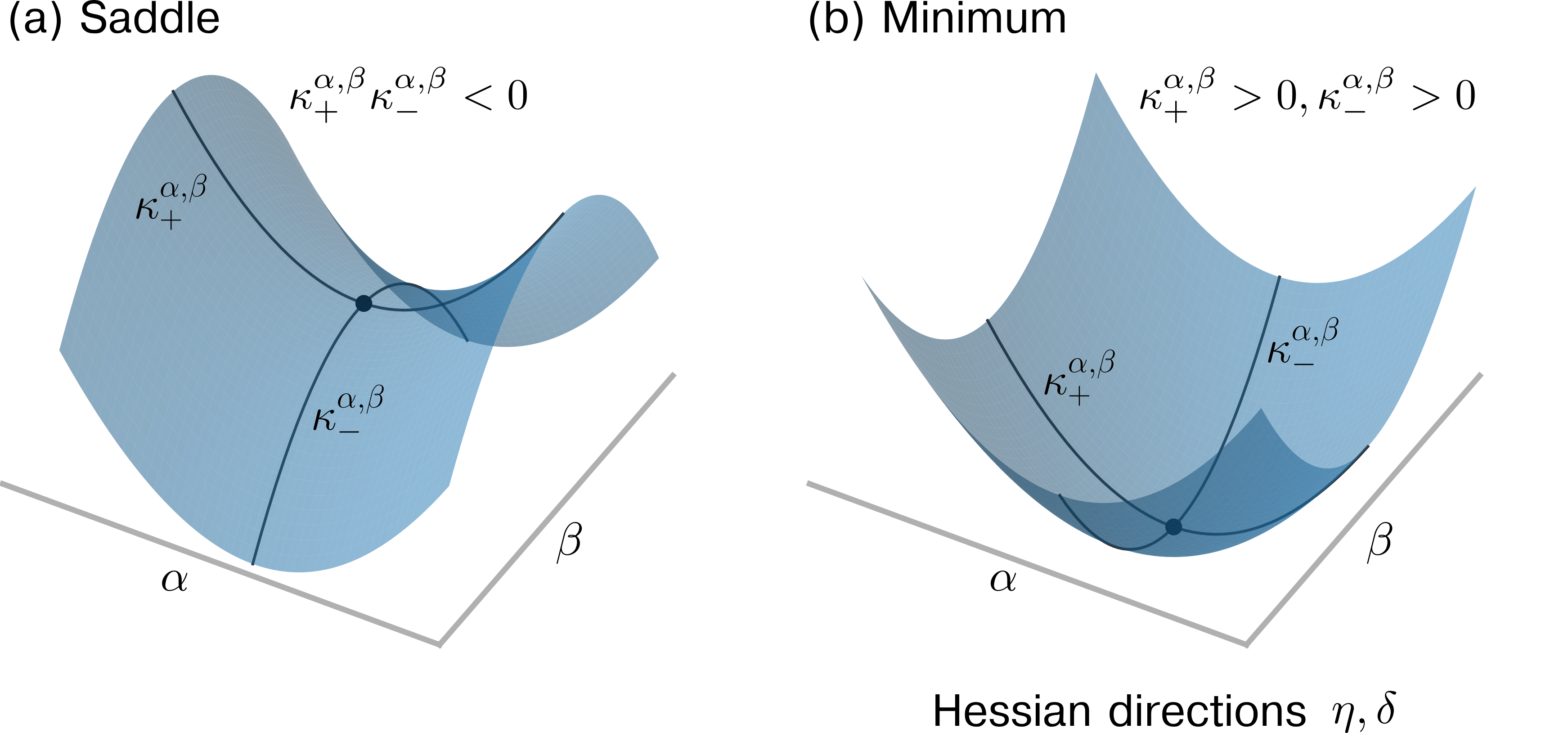
\n ## Diagram: Saddle Point and Minimum Illustration ### Overview The image presents two 3D diagrams illustrating the concepts of a saddle point (a) and a minimum (b) in a two-dimensional space defined by axes α and β. Both diagrams depict a curved surface, with annotations indicating curvature values. The diagrams are side-by-side for comparison. ### Components/Axes * **Axes:** Both diagrams share the same axes labeled α (x-axis) and β (y-axis). * **Curvature Labels:** Each diagram features two curvature labels: κ^α,β₊ and κ^α,β_-. These labels are positioned on the curved surface to indicate the direction of curvature. * **Conditions:** Each diagram includes a mathematical condition relating the curvature values: * **(a) Saddle:** κ^α,β₊ κ^α,β_- < 0 * **(b) Minimum:** κ^α,β₊ > 0, κ^α,β_- > 0 * **Hessian Directions:** Below the second diagram, the text "Hessian directions η, δ" is present. ### Detailed Analysis / Content Details **Diagram (a) - Saddle Point:** * The surface resembles a saddle, with upward curvature along the α-axis and downward curvature along the β-axis. * The label κ^α,β₊ is positioned on the upward-curving portion of the surface, near the α-axis. * The label κ^α,β_- is positioned on the downward-curving portion of the surface, near the β-axis. * The condition κ^α,β₊ κ^α,β_- < 0 indicates that the product of the curvatures is negative, which is characteristic of a saddle point. **Diagram (b) - Minimum:** * The surface curves upwards in both the α and β directions, forming a bowl-like shape. * The label κ^α,β₊ is positioned on the upward-curving portion of the surface, near the α-axis. * The label κ^α,β_- is positioned on the upward-curving portion of the surface, near the β-axis. * The condition κ^α,β₊ > 0, κ^α,β_- > 0 indicates that both curvatures are positive, which is characteristic of a minimum. ### Key Observations * The diagrams visually demonstrate the difference between a saddle point and a minimum. * The curvature labels and conditions provide a mathematical description of these concepts. * The Hessian directions are mentioned, suggesting a connection to the Hessian matrix used in optimization problems. * The diagrams are simplified representations, focusing on the curvature rather than precise numerical values. ### Interpretation The diagrams illustrate fundamental concepts in multivariable calculus and optimization. The saddle point represents a critical point where the function has zero gradient, but it is not a local minimum or maximum. The minimum represents a point where the function reaches its lowest value in a local region. The curvature values (κ^α,β₊ and κ^α,β_-) quantify the rate of change of the function along the α and β axes, respectively. The conditions provided relate these curvature values to the type of critical point. The mention of Hessian directions suggests that these diagrams are relevant to the second derivative test, which uses the Hessian matrix to determine the nature of critical points. The diagrams are useful for visualizing these abstract concepts and understanding their geometric interpretation.