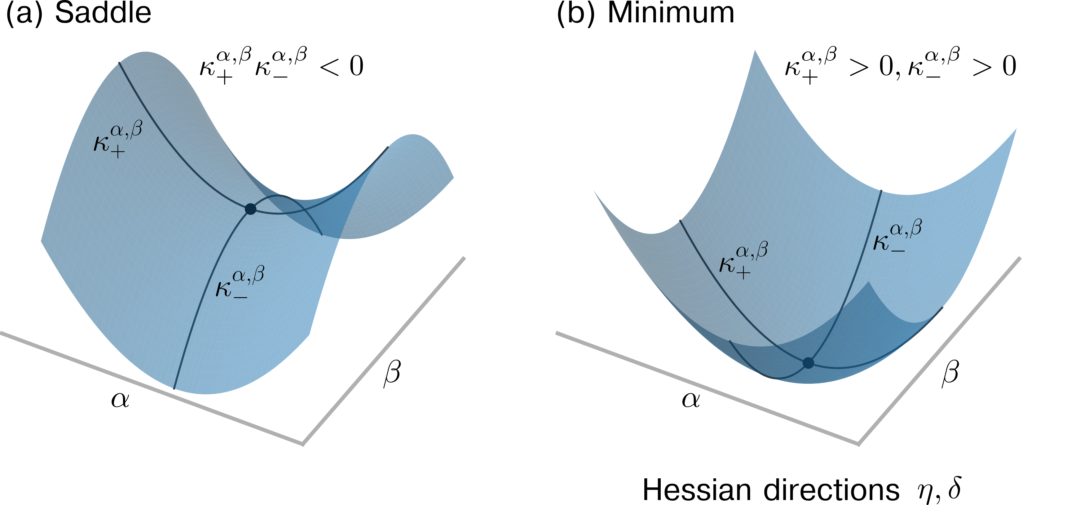
## 3D Function Visualization: Saddle Point vs. Minimum ### Overview The image contains two 3D surface plots comparing critical points in a multivariable function. Plot (a) shows a saddle point configuration, while plot (b) illustrates a minimum point. Both plots use α and β as independent variables on orthogonal axes, with implicit third-axis values representing function output. ### Components/Axes - **Axes Labels**: - Horizontal axes: α (x-axis), β (y-axis) - Vertical axis: Implicit function value (z-axis) - **Mathematical Labels**: - κ+α,β and κ−α,β annotations on both plots - Hessian directions η, δ labeled at bottom of plot (b) - **Color Coding**: - Light blue shading for surface areas - Dark blue lines for critical point contours - Black dots marking critical points ### Detailed Analysis #### Plot (a) Saddle Point - **Surface Structure**: - Hyperbolic paraboloid shape with opposing curvature - Central black dot at intersection of κ+ and κ− contours - **Mathematical Conditions**: - κ+α,β < 0 and κ−α,β < 0 (both negative definite) - Critical point occurs where surface crosses itself - **Spatial Features**: - Left side shows upward curvature (α-direction) - Right side shows downward curvature (β-direction) #### Plot (b) Minimum - **Surface Structure**: - Parabolic bowl shape with single global minimum - Central black dot at lowest point - **Mathematical Conditions**: - κ+α,β > 0 and κ−α,β > 0 (both positive definite) - Hessian directions η, δ indicate gradient paths - **Spatial Features**: - All directions curve upward from central minimum - Contour lines form concentric ellipses around minimum ### Key Observations 1. **Curvature Sign Relationship**: - Saddle point (a) shows mixed curvature signs (one positive, one negative) - Minimum (b) shows uniform positive curvature 2. **Hessian Directionality**: - Only present in minimum plot (b) - Arrows point toward minimum along principal axes 3. **Critical Point Identification**: - Saddle point marked by intersecting surface - Minimum marked by lowest surface point 4. **Symmetry**: - Both plots show bilateral symmetry about α=0 and β=0 ### Interpretation The visualization demonstrates fundamental concepts in multivariable calculus: 1. **Saddle Point Significance**: - Represents unstable equilibrium where function increases in one direction and decreases in another - Mathematical manifestation of competing gradients 2. **Minimum Characteristics**: - Stable equilibrium point with positive definite Hessian - Indicates local/global optimization target 3. **Hessian Geometry**: - Directions η, δ in plot (b) show paths of steepest descent - Elliptical contour patterns confirm quadratic approximation validity 4. **Practical Implications**: - Saddle points often represent transition states in physical systems - Minima correspond to equilibrium states in optimization problems - Curvature analysis provides insight into function behavior near critical points The plots effectively demonstrate how second derivative information (Hessian matrix) determines the nature of critical points through curvature analysis.