## Diagram: LLM Fine-Tuning and DFS Inference
### Overview
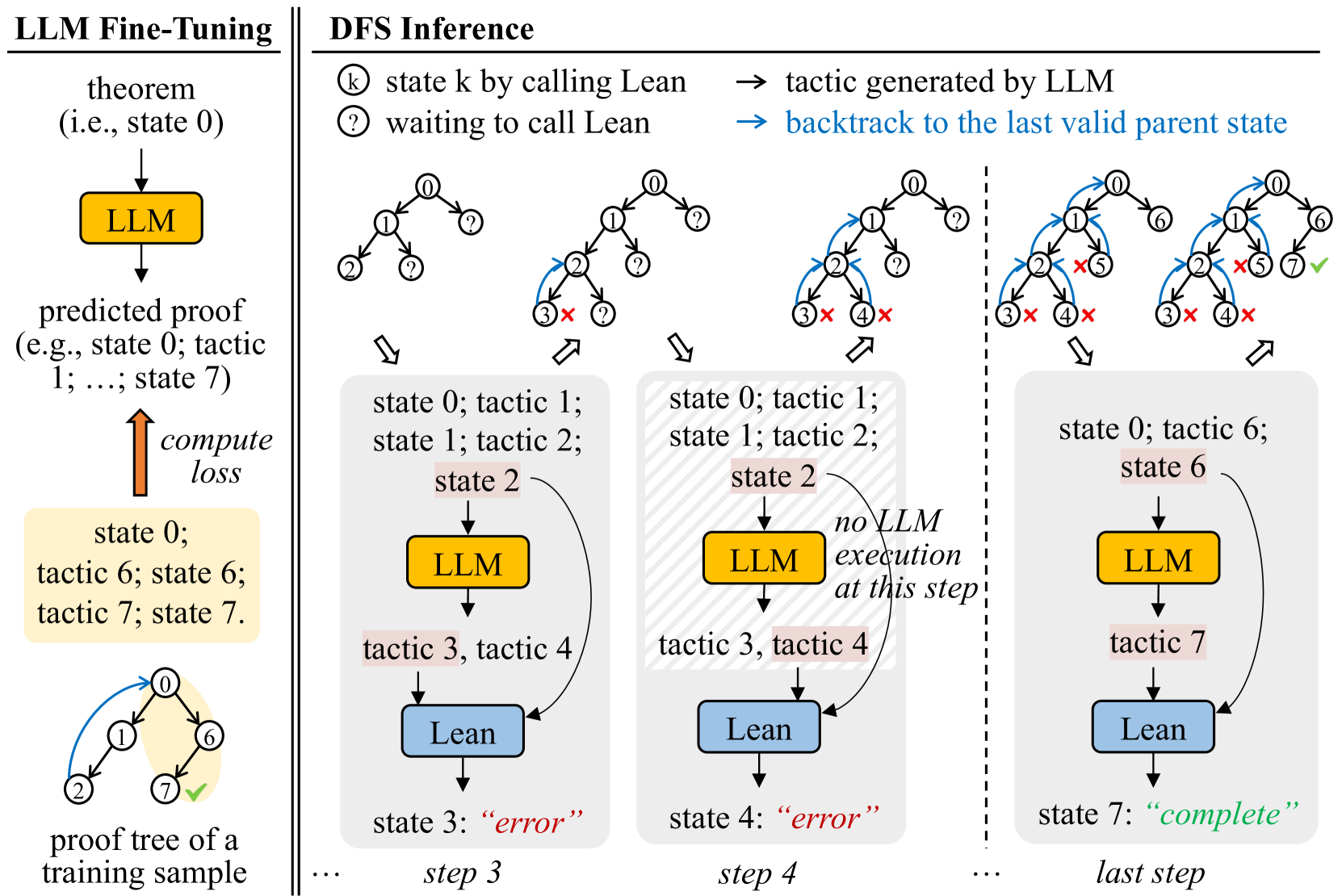
The image illustrates a comparison between LLM fine-tuning and Depth-First Search (DFS) inference in the context of automated theorem proving. The left side depicts the fine-tuning process, while the right side demonstrates the DFS inference process with LLM assistance.
### Components/Axes
**Left Side: LLM Fine-Tuning**
* **Title:** LLM Fine-Tuning
* **Elements:**
* "theorem (i.e., state 0)" with a downward arrow.
* Yellow box labeled "LLM".
* "predicted proof (e.g., state 0; tactic 1; ...; state 7)" below the LLM box.
* Upward arrow labeled "compute loss".
* Yellow box containing "state 0; tactic 6; state 6; tactic 7; state 7".
* A tree diagram with nodes labeled 0, 1, 2, 6, and 7. Node 7 has a green checkmark.
* Label: "proof tree of a training sample"
**Right Side: DFS Inference**
* **Title:** DFS Inference
* **Legend (Top-Right):**
* "state k by calling Lean" (circle with 'k' inside)
* "waiting to call Lean" (circle with '?')"
* "tactic generated by LLM" (rightward arrow)
* "backtrack to the last valid parent state" (blue rightward arrow)
* **Elements:**
* Four tree diagrams representing different steps in the DFS inference process.
* Boxes below each tree diagram representing the current state and actions.
* Yellow boxes labeled "LLM".
* Blue boxes labeled "Lean".
* Arrows indicating the flow of information between LLM and Lean.
* Labels indicating the state and tactics at each step.
* Labels indicating the outcome of each step ("error" or "complete").
* Labels indicating the step number (step 3, step 4, last step).
### Detailed Analysis
**LLM Fine-Tuning (Left Side):**
* The process starts with a theorem (state 0).
* The LLM predicts a proof.
* The predicted proof is compared to the ground truth, and a loss is computed.
* The loss is used to fine-tune the LLM.
* The example shows a proof tree with nodes 0, 1, 2, 6, and 7. Node 7 is marked as complete.
**DFS Inference (Right Side):**
* **Step 1 (Implied):** The initial tree has node 0 and question marks on the children.
* **Step 2 (Implied):** The tree expands with nodes 1 and 2. Node 3 has a red 'X', indicating an error.
* **Step 3:**
* Tree: Nodes 0, 1, 2, 3 (marked with a red 'X'), and 4 (marked with a red 'X').
* State: "state 0; tactic 1; state 1; tactic 2; state 2"
* LLM: Yellow box labeled "LLM".
* Tactics: "tactic 3, tactic 4"
* Lean: Blue box labeled "Lean".
* Outcome: "state 3: 'error'"
* **Step 4:**
* Tree: Nodes 0, 1, 2, 3 (marked with a red 'X'), and 4 (marked with a red 'X').
* State: "state 0; tactic 1; state 1; tactic 2; state 2"
* LLM: Yellow box labeled "LLM".
* Text: "no LLM execution at this step!"
* Tactics: "tactic 3, tactic 4"
* Lean: Blue box labeled "Lean".
* Outcome: "state 4: 'error'"
* **Last Step:**
* Tree: Nodes 0, 1, 2, 3 (marked with a red 'X'), 4 (marked with a red 'X'), 5 (marked with a red 'X'), 6, and 7 (marked with a green checkmark).
* State: "state 0; tactic 6; state 6"
* LLM: Yellow box labeled "LLM".
* Tactics: "tactic 7"
* Lean: Blue box labeled "Lean".
* Outcome: "state 7: 'complete'"
### Key Observations
* The DFS inference process involves exploring different proof paths.
* The LLM suggests tactics to try at each step.
* If a tactic leads to an error, the algorithm backtracks to the last valid parent state.
* The process continues until a complete proof is found.
### Interpretation
The diagram illustrates how an LLM can be used to assist in automated theorem proving. The LLM is first fine-tuned on a dataset of proofs. Then, during the DFS inference process, the LLM suggests tactics to try at each step. This can help to guide the search for a proof and reduce the amount of time it takes to find a solution. The diagram highlights the iterative nature of the DFS inference process, with the algorithm backtracking when it encounters an error and continuing until a complete proof is found. The "no LLM execution at this step!" text suggests that sometimes the system relies on pre-programmed or deterministic steps, rather than always querying the LLM.