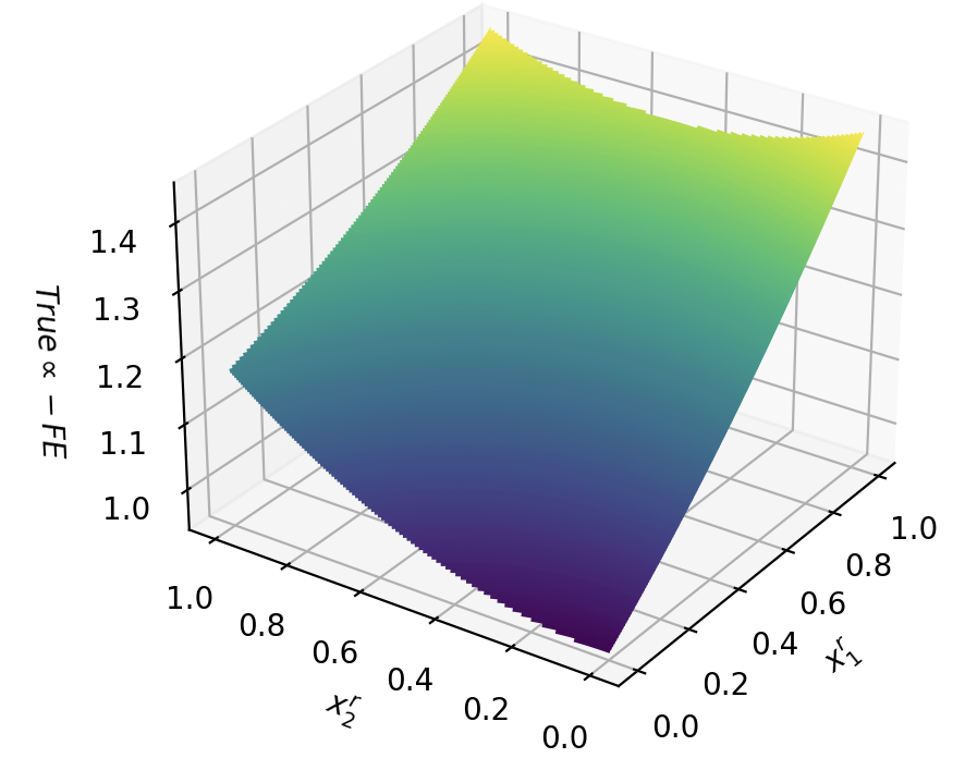
\n ## 3D Surface Plot: Relationship of "True α - FE" with Normalized Parameters x̃₁ and x̃₂ ### Overview The image displays a three-dimensional surface plot. The plot visualizes how a dependent variable, labeled "True α - FE", changes as a function of two independent, normalized variables, "x̃₁" and "x̃₂". The surface is rendered with a color gradient that maps the value of the vertical axis. ### Components/Axes * **Vertical Axis (Z-axis):** * **Label:** `True α - FE` * **Scale:** Linear, ranging from 1.0 to 1.4. * **Tick Marks:** 1.0, 1.1, 1.2, 1.3, 1.4. * **Horizontal Axis 1 (X-axis, front-left):** * **Label:** `x̃₁` (x-tilde sub 1) * **Scale:** Linear, ranging from 0.0 to 1.0. * **Tick Marks:** 0.0, 0.2, 0.4, 0.6, 0.8, 1.0. * **Horizontal Axis 2 (Y-axis, front-right):** * **Label:** `x̃₂` (x-tilde sub 2) * **Scale:** Linear, ranging from 0.0 to 1.0. * **Tick Marks:** 0.0, 0.2, 0.4, 0.6, 0.8, 1.0. * **Color Mapping:** The surface color corresponds to the Z-axis value (`True α - FE`). A gradient is used, transitioning from dark purple/blue for the lowest values (~1.0) through teal and green to bright yellow for the highest values (~1.4). There is no separate legend; the color is an intrinsic part of the data surface. ### Detailed Analysis * **Surface Shape and Trend:** The surface forms a smooth, continuous, and slightly curved plane. It exhibits a clear monotonic trend in both horizontal dimensions. * **Trend with x̃₁:** For any fixed value of x̃₂, the surface slopes **upward** as x̃₁ increases from 0.0 to 1.0. This indicates a positive correlation between `True α - FE` and x̃₁. * **Trend with x̃₂:** For any fixed value of x̃₁, the surface slopes **downward** as x̃₂ increases from 0.0 to 1.0. This indicates a negative correlation between `True α - FE` and x̃₂. * **Data Point Approximation (Spatial Grounding):** * **Minimum Region:** The lowest point on the surface (dark purple) is located at the corner where **x̃₁ is near 0.0 and x̃₂ is near 1.0**. The corresponding `True α - FE` value is approximately **1.0**. * **Maximum Region:** The highest point on the surface (bright yellow) is located at the opposite corner where **x̃₁ is near 1.0 and x̃₂ is near 0.0**. The corresponding `True α - FE` value is approximately **1.4**. * **Intermediate Values:** The surface passes through intermediate values smoothly. For example, at the center point (x̃₁=0.5, x̃₂=0.5), the color is a medium green, suggesting a `True α - FE` value of approximately **1.2**. ### Key Observations 1. **Linear-like Relationship:** The surface appears largely planar, suggesting the relationship between `True α - FE` and the two parameters (x̃₁, x̃₂) may be approximately linear or bilinear within this domain. There is no strong curvature indicating a complex, non-linear interaction. 2. **Dominant Effect of x̃₁:** The gradient of the surface appears steeper along the x̃₁ direction compared to the x̃₂ direction. This suggests that changes in x̃₁ have a stronger influence on the output variable `True α - FE` than equivalent changes in x̃₂. 3. **No Interaction Effect:** The surface does not exhibit twisting or saddle-like behavior. The effect of changing x̃₁ appears consistent regardless of the value of x̃₂, and vice-versa. This implies the two parameters likely influence the output independently (additively) rather than through a multiplicative interaction. ### Interpretation This plot is a response surface, likely generated from a computational model or experimental design. It maps the output `True α - FE` (which could represent a true value minus a finite element approximation, a common error metric in numerical analysis) across a normalized parameter space defined by x̃₁ and x̃₂. The data demonstrates that the error or quantity `True α - FE` is minimized (approaches 1.0) when parameter x̃₁ is low and x̃₂ is high. Conversely, it is maximized (approaches 1.4) when x̃₁ is high and x̃₂ is low. The near-planar shape indicates a predictable, systematic relationship. The stronger dependence on x̃₁ suggests it is the more critical parameter to control or understand for predicting the value of `True α - FE`. This type of visualization is crucial in sensitivity analysis, optimization, and understanding model behavior across a multi-dimensional input space.