## 3D Surface Plot: True α – FE vs. x₁ and x₂
### Overview
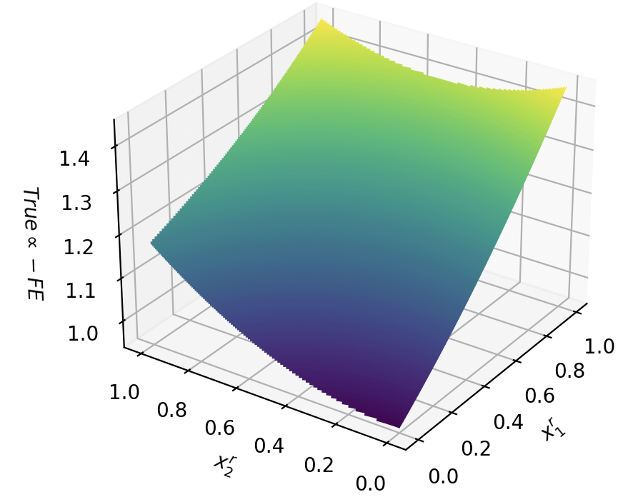
The image depicts a 3D surface plot visualizing the relationship between two input variables (`x₁` and `x₂`) and a response variable (`True α – FE`). The surface is colored using a gradient from purple (low values) to yellow (high values), with a grid background providing spatial reference. The plot shows a smooth, curved surface with a peak at the top-right corner.
---
### Components/Axes
1. **Axes Labels**:
- **x₁ (horizontal axis)**: Ranges from 0.0 to 1.0 in increments of 0.2.
- **x₂ (depth axis)**: Ranges from 0.0 to 1.0 in increments of 0.2.
- **True α – FE (vertical axis)**: Ranges from 1.0 to 1.4 in increments of 0.1.
2. **Color Gradient**:
- **Purple**: Represents the lowest values of `True α – FE` (~1.0).
- **Yellow**: Represents the highest values of `True α – FE` (~1.4).
- **Green/Blue**: Intermediate values (~1.1–1.3).
3. **Grid**:
- A 3D grid spans the background, with lines spaced evenly along all axes.
---
### Detailed Analysis
- **Surface Shape**:
- The surface is smooth and curved, with a pronounced peak at the top-right corner (x₁ = 1.0, x₂ = 1.0).
- The gradient transitions from purple (bottom-left) to yellow (top-right), indicating increasing `True α – FE` values as `x₁` and `x₂` increase.
- **Key Data Points**:
- At (x₁ = 0.0, x₂ = 0.0): `True α – FE` ≈ 1.0 (purple).
- At (x₁ = 1.0, x₂ = 1.0): `True α – FE` ≈ 1.4 (yellow).
- Intermediate values (e.g., x₁ = 0.5, x₂ = 0.5): `True α – FE` ≈ 1.2–1.3 (green/blue).
- **Color Consistency**:
- The color gradient aligns with the vertical axis scale, confirming that higher `True α – FE` values correspond to warmer colors (yellow).
---
### Key Observations
1. **Peak at Maximum Inputs**:
- The highest `True α – FE` value (1.4) occurs when both `x₁` and `x₂` are at their maximum (1.0).
2. **Gradual Increase**:
- `True α – FE` increases monotonically as `x₁` and `x₂` increase, with no visible plateaus or anomalies.
3. **Smooth Gradient**:
- The color transition is continuous, suggesting a linear or near-linear relationship between inputs and the response.
---
### Interpretation
The plot demonstrates that `True α – FE` is directly influenced by both `x₁` and `x₂`, with the strongest effect observed when both variables are maximized. The smooth surface and gradient imply a predictable, non-linear relationship between the inputs and the response. The absence of outliers or discontinuities suggests a well-behaved system, where small changes in `x₁` and `x₂` lead to proportional changes in `True α – FE`. This could represent a physical or mathematical model where efficiency (`α`) or error (`FE`) is optimized at extreme input values.