# Technical Data Extraction: Conductance vs. Twisting Angle in Transition Metal Dichalcogenides
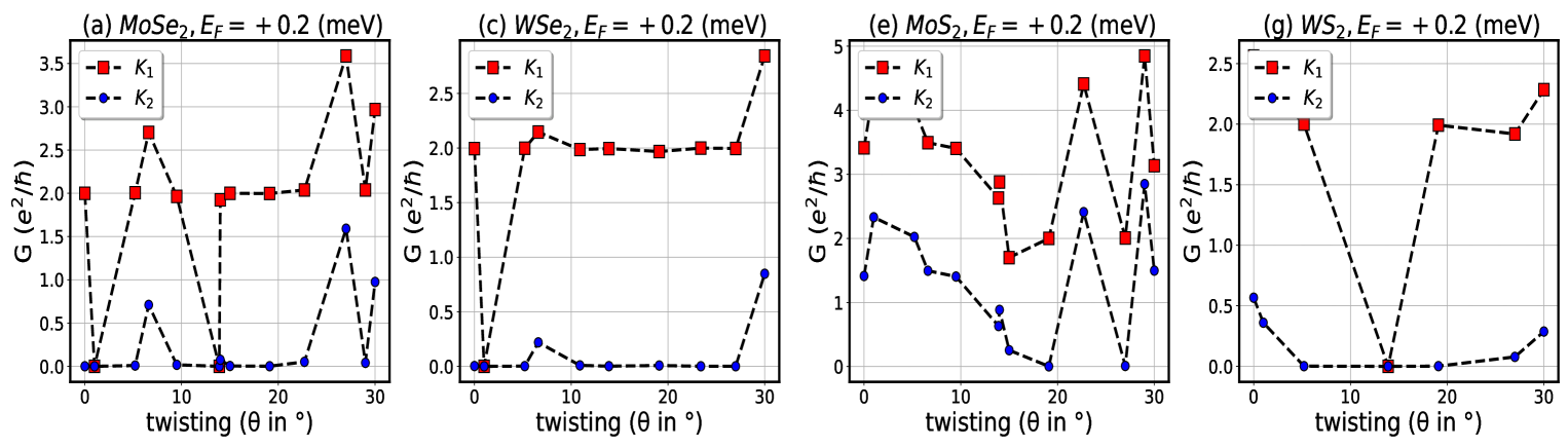
This document provides a comprehensive extraction of data from a series of four scientific plots showing the relationship between conductance ($G$) and twisting angle ($\theta$) for different materials at a specific Fermi energy ($E_F = +0.2$ meV).
## 1. General Metadata and Global Parameters
* **Image Type:** Multi-panel line graph (4 panels).
* **Common X-axis:** twisting ($\theta$ in $^\circ$). Range: 0 to 30.
* **Common Y-axis:** $G$ ($e^2/h$). Range varies by panel.
* **Common Legend:**
* **Red Squares (dashed line):** $K_1$ (Valley 1)
* **Blue Circles (dashed line):** $K_2$ (Valley 2)
* **Fermi Energy ($E_F$):** Constant at $+0.2$ meV for all panels.
* **Language:** English.
---
## 2. Panel Analysis
### Panel (a): $MoSe_2$
* **Header:** (a) $MoSe_2, E_F = +0.2$ (meV)
* **Y-axis Range:** 0.0 to 3.5+
* **Trend Analysis:**
* **$K_1$ (Red):** Starts at 2.0, fluctuates significantly with sharp peaks at $\sim 7^\circ$ and $\sim 27^\circ$. It drops to near zero at $\sim 14^\circ$.
* **$K_2$ (Blue):** Remains very low (near 0) for most angles, with small peaks at $\sim 7^\circ$ and a significant spike to $\sim 1.6$ at $\sim 27^\circ$.
* **Approximate Data Points:**
* $\theta \approx 0$: $K_1 \approx 2.0, K_2 \approx 0.0$
* $\theta \approx 7$: $K_1 \approx 2.7, K_2 \approx 0.7$
* $\theta \approx 14$: $K_1 \approx 0.0, K_2 \approx 0.0$
* $\theta \approx 27$: $K_1 \approx 3.6, K_2 \approx 1.6$
* $\theta \approx 30$: $K_1 \approx 3.0, K_2 \approx 1.0$
### Panel (c): $WSe_2$
* **Header:** (c) $WSe_2, E_F = +0.2$ (meV)
* **Y-axis Range:** 0.0 to 2.5+
* **Trend Analysis:**
* **$K_1$ (Red):** Shows a "plateau" behavior. After an initial drop at $1^\circ$, it stays remarkably stable near $G=2.0$ from $5^\circ$ to $27^\circ$, before spiking at $30^\circ$.
* **$K_2$ (Blue):** Almost entirely suppressed (near 0) across the whole range, except for a small rise at $30^\circ$.
* **Approximate Data Points:**
* $\theta \approx 0$: $K_1 \approx 2.0, K_2 \approx 0.0$
* $\theta \approx 1$: $K_1 \approx 0.0, K_2 \approx 0.0$
* $\theta \approx 10-25$: $K_1 \approx 2.0, K_2 \approx 0.0$
* $\theta \approx 30$: $K_1 \approx 2.8, K_2 \approx 0.8$
### Panel (e): $MoS_2$
* **Header:** (e) $MoS_2, E_F = +0.2$ (meV)
* **Y-axis Range:** 0 to 5
* **Trend Analysis:**
* **$K_1$ (Red):** Highly oscillatory. High values ($>3$) at low angles, a dip near $15^\circ$, a massive peak at $\sim 23^\circ$, another dip, and a final peak at $29^\circ$.
* **$K_2$ (Blue):** Follows a similar oscillatory pattern to $K_1$ but at a lower magnitude (generally between 0 and 2.5).
* **Approximate Data Points:**
* $\theta \approx 0$: $K_1 \approx 3.4, K_2 \approx 1.4$
* $\theta \approx 15$: $K_1 \approx 1.7, K_2 \approx 0.3$
* $\theta \approx 23$: $K_1 \approx 4.4, K_2 \approx 2.4$
* $\theta \approx 29$: $K_1 \approx 4.8, K_2 \approx 2.8$
### Panel (g): $WS_2$
* **Header:** (g) $WS_2, E_F = +0.2$ (meV)
* **Y-axis Range:** 0.0 to 2.5
* **Trend Analysis:**
* **$K_1$ (Red):** Data is missing for low angles ($<5^\circ$). It starts high at $\sim 2.0$, drops to zero at the midpoint ($\sim 14^\circ$), then recovers to $\sim 2.0$ and stays relatively flat until a final rise at $30^\circ$.
* **$K_2$ (Blue):** Starts at $\sim 0.6$, decays to zero by $5^\circ$, stays at zero until $\sim 25^\circ$, then rises slightly.
* **Approximate Data Points:**
* $\theta \approx 0$: $K_1 = \text{N/A}, K_2 \approx 0.6$
* $\theta \approx 5$: $K_1 \approx 2.0, K_2 \approx 0.0$
* $\theta \approx 14$: $K_1 \approx 0.0, K_2 \approx 0.0$
* $\theta \approx 20$: $K_1 \approx 2.0, K_2 \approx 0.0$
* $\theta \approx 30$: $K_1 \approx 2.3, K_2 \approx 0.3$
---
## 3. Component Isolation Summary
| Region | Content Description |
| :--- | :--- |
| **Header** | Contains panel labels (a, c, e, g) and material/energy specs. |
| **Main Chart Area** | Four sub-plots with dashed lines connecting data points. Grid lines are present. |
| **Legend** | Located in the top-left of each sub-plot. Red Square = $K_1$, Blue Circle = $K_2$. |
| **Footer** | Contains the X-axis label "twisting ($\theta$ in $^\circ$)" repeated for each column. |
## 4. Key Observations
1. **Symmetry/Dips:** Most materials show a significant drop in conductance ($G \rightarrow 0$) near the middle of the angular range (around $14^\circ - 15^\circ$).
2. **Valley Dominance:** In almost all cases, the $K_1$ valley (red) contributes significantly more to the total conductance than the $K_2$ valley (blue).
3. **Material Variation:** $MoS_2$ exhibits the highest absolute conductance values (peaking near 5 $e^2/h$), while $WSe_2$ shows the most stable conductance plateau.