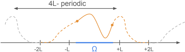
## Line Graph: 4L-Periodic vs Continuous Function ### Overview The image depicts a line graph comparing two functions over a symmetric interval from -2L to +2L on the x-axis. The graph includes a periodic function (orange, solid line) and a continuous function (gray, dashed line), with key features annotated and labeled. --- ### Components/Axes - **X-axis**: Labeled with positions -2L, -L, 0, +L, +2L. Represents spatial or temporal intervals. - **Y-axis**: Labeled Ω (Greek letter omega), likely representing a variable such as angular frequency, amplitude, or another physical quantity. - **Legend**: Located at the top of the graph. - **Orange (solid line)**: Labeled "4L-periodic". - **Gray (dashed line)**: Labeled "Continuous". --- ### Detailed Analysis 1. **4L-Periodic Function (Orange, Solid Line)**: - **Peaks**: Two distinct peaks at x = -L and x = +L, with a trough at x = 0. - **Periodicity**: Repeats every 4L units (e.g., from -2L to +2L spans one full period). - **Amplitude**: Higher peaks compared to the continuous function. - **Symmetry**: Symmetric about the y-axis (even function). 2. **Continuous Function (Gray, Dashed Line)**: - **Peaks**: Two peaks at x = -2L and x = +2L, with a trough at x = 0. - **Behavior**: Smooth, non-repeating curve with no periodicity. - **Amplitude**: Lower peaks compared to the periodic function. 3. **Key Data Points**: - At x = -2L: Gray line starts at a peak (Ω ≈ 1.0), orange line at baseline (Ω ≈ 0). - At x = -L: Orange line peaks (Ω ≈ 1.2), gray line at Ω ≈ 0.5. - At x = 0: Both lines cross at Ω ≈ 0 (trough). - At x = +L: Orange line peaks again (Ω ≈ 1.2), gray line at Ω ≈ 0.5. - At x = +2L: Gray line peaks (Ω ≈ 1.0), orange line returns to baseline. --- ### Key Observations - The **4L-periodic function** exhibits regular oscillations with peaks at ±L and a trough at 0, consistent with a sinusoidal or square-wave-like behavior. - The **continuous function** lacks periodicity but shows peaks at the extremes (±2L), suggesting a different underlying mechanism (e.g., boundary-driven or decaying behavior). - The **amplitude difference** between the two functions highlights distinct characteristics: the periodic function has sharper, higher peaks, while the continuous function’s peaks are broader and lower. - Both functions share a **trough at x = 0**, indicating a shared symmetry or boundary condition. --- ### Interpretation - **Physical/Technical Context**: The graph likely models a system with periodic and non-periodic components. For example: - The **4L-periodic function** could represent a wave or signal with a fixed wavelength (e.g., a standing wave in a medium of length 2L). - The **continuous function** might model a transient or boundary-affected phenomenon (e.g., a decaying oscillation or a function constrained by endpoints). - **Relationships**: - The periodic function’s peaks at ±L suggest a **half-period** alignment with the interval’s midpoint (0), while the continuous function’s peaks at ±2L align with the interval’s endpoints. - The shared trough at 0 implies a **node** or equilibrium point common to both functions. - **Anomalies/Outliers**: None observed. Both functions behave predictably within their defined characteristics. --- ### Conclusion The graph illustrates a fundamental contrast between periodic and continuous behaviors in a system. The 4L-periodic function’s regularity and symmetry contrast with the continuous function’s endpoint-driven peaks, offering insights into phenomena such as resonance, wave propagation, or boundary conditions in physical or mathematical systems.