## Chart: Phase Space Visualization of Dynamical Systems
### Overview
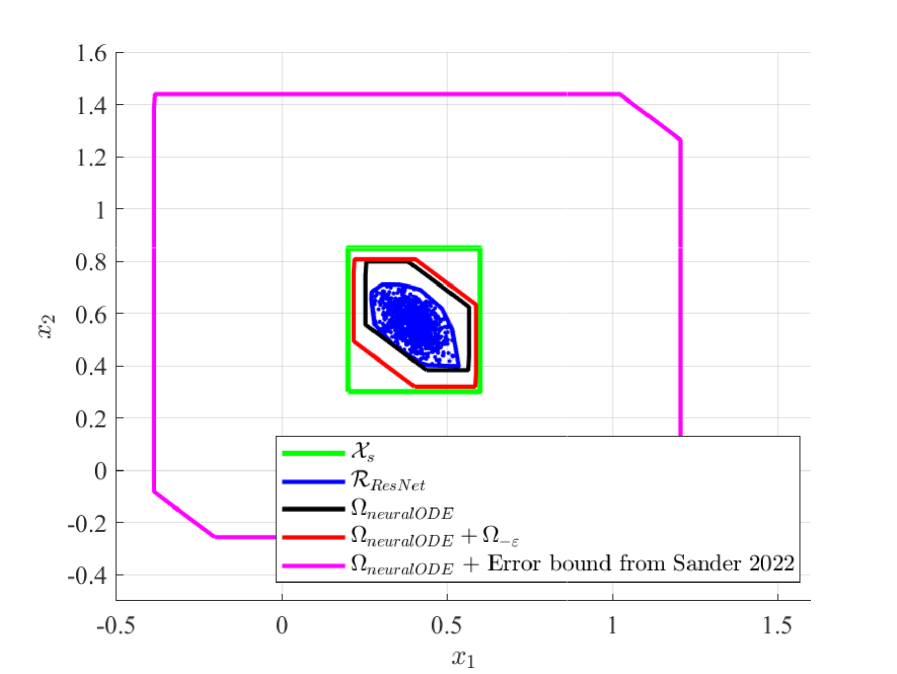
The image presents a 2D phase space plot, likely representing the trajectories of dynamical systems. The plot visualizes the state space defined by variables x₁ and x₂. Several curves are overlaid, each representing a different method or model for approximating the system's behavior. The plot appears to be comparing the performance of different numerical integration schemes or models in capturing the true dynamics.
### Components/Axes
* **x-axis:** Labeled "x₁", ranging approximately from -0.5 to 1.5.
* **y-axis:** Labeled "x₂", ranging approximately from -0.4 to 1.6.
* **Legend:** Located in the bottom-left corner, listing the following curves and their corresponding colors:
* χs (Green)
* RResNet (Dark Blue)
* ΩneuralODE (Red)
* ΩneuralODE + Ωε (Black)
* ΩneuralODE + Error bound from Sander 2022 (Magenta)
### Detailed Analysis
The plot shows several closed curves, indicating potentially periodic or bounded behavior of the dynamical systems.
* **χs (Green):** This curve forms a roughly rectangular shape. It starts at approximately (-0.5, 0.8), goes to (0.5, 0.8), then to (0.5, 1.4), then to (-0.5, 1.4), and back to the starting point.
* **RResNet (Dark Blue):** This curve is contained within the green curve and appears more complex, with several lobes and indentations. It roughly follows a similar overall shape to the green curve, but with more oscillations. The curve starts at approximately (0.0, 0.6), moves to (0.4, 0.7), then to (0.6, 0.5), then to (0.2, 0.3), and back to the starting point.
* **ΩneuralODE (Red):** This curve is also contained within the green curve and appears to be smoother than the RResNet curve. It starts at approximately (0.0, 0.5), moves to (0.5, 0.6), then to (0.7, 0.4), then to (0.3, 0.2), and back to the starting point.
* **ΩneuralODE + Ωε (Black):** This curve is very similar to the red curve, but slightly offset. It starts at approximately (0.0, 0.4), moves to (0.5, 0.5), then to (0.7, 0.3), then to (0.3, 0.1), and back to the starting point.
* **ΩneuralODE + Error bound from Sander 2022 (Magenta):** This curve forms the outer boundary of the region, encompassing all other curves. It starts at approximately (-0.5, -0.2), moves to (1.5, 1.4), then to (1.5, -0.2), and back to the starting point.
### Key Observations
* The magenta curve (ΩneuralODE + Error bound from Sander 2022) represents the widest region, suggesting it provides the most conservative estimate of the system's behavior.
* The green curve (χs) defines a relatively simple, rectangular boundary.
* The RResNet and ΩneuralODE curves are contained within the green curve, indicating they provide more refined approximations.
* The black curve (ΩneuralODE + Ωε) is very close to the red curve (ΩneuralODE), suggesting that the addition of Ωε has a relatively small effect.
* The RResNet curve exhibits more complex oscillations than the ΩneuralODE curve.
### Interpretation
This plot likely compares the accuracy and robustness of different methods for solving or approximating a dynamical system. The green curve might represent a known or "true" solution, while the other curves represent approximations obtained using different numerical methods or models. The magenta curve represents the true solution plus an error bound.
The fact that the RResNet and ΩneuralODE curves are contained within the green curve suggests that these methods are providing reasonable approximations. The differences between the curves highlight the trade-offs between accuracy, computational cost, and robustness. The RResNet curve's more complex shape suggests it might be capturing finer details of the dynamics, but it could also be more sensitive to noise or errors. The error bound (magenta curve) provides a measure of the uncertainty associated with the ΩneuralODE approximation.
The reference to "Sander 2022" suggests that the error bound is based on results published in that paper. This plot is a visual representation of the performance of these methods in a specific phase space, and it could be used to guide the selection of an appropriate method for a given application.