## State-Space Diagram: Comparison of Invariant and Reachable Sets
### Overview
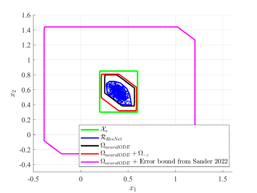
The image is a 2D state-space plot (phase portrait) comparing different computed sets for a dynamical system. It visualizes the relationship between a reachable set from a ResNet model (`R_ResNet`) and several invariant set approximations (`Ω_neuralODE`) with different error bounds. The plot demonstrates how conservative various bounding methods are relative to each other and to the computed reachable set.
### Components/Axes
* **Chart Type:** 2D State-Space / Phase Portrait Diagram.
* **Axes:**
* **X-axis:** Labeled `x₁`. Scale ranges from approximately -0.5 to 1.5, with major ticks at -0.5, 0, 0.5, 1, 1.5.
* **Y-axis:** Labeled `x₂`. Scale ranges from approximately -0.4 to 1.6, with major ticks at -0.4, -0.2, 0, 0.2, 0.4, 0.6, 0.8, 1, 1.2, 1.4, 1.6.
* **Legend:** Positioned at the bottom-center of the plot area. It contains five entries, each with a colored line sample and a corresponding label:
1. **Green Line:** `Xₛ`
2. **Blue Line:** `R_ResNet`
3. **Black Line:** `Ω_neuralODE`
4. **Red Line:** `Ω_neuralODE + Ω₋ₑ`
5. **Magenta Line:** `Ω_neuralODE + Error bound from Sander 2022`
### Detailed Analysis
The diagram contains five distinct geometric regions, nested within each other. Their spatial relationships and approximate coordinates are as follows:
1. **Magenta Polygon (`Ω_neuralODE + Error bound from Sander 2022`):**
* **Trend/Shape:** This is the outermost, largest polygon. It is an irregular hexagon.
* **Approximate Vertices (x₁, x₂):** (-0.4, -0.1), (-0.2, -0.25), (1.2, -0.25), (1.2, 1.25), (1.0, 1.45), (-0.4, 1.45). It encloses all other shapes.
2. **Green Rectangle (`Xₛ`):**
* **Trend/Shape:** A simple axis-aligned rectangle nested inside the magenta polygon.
* **Approximate Bounds:** x₁ from ~0.2 to ~0.6; x₂ from ~0.3 to ~0.8.
3. **Red Polygon (`Ω_neuralODE + Ω₋ₑ`):**
* **Trend/Shape:** An irregular hexagon nested inside the green rectangle. It is smaller than the green rectangle but larger than the black polygon.
* **Approximate Vertices (x₁, x₂):** (0.25, 0.3), (0.25, 0.6), (0.35, 0.7), (0.55, 0.6), (0.55, 0.3), (0.35, 0.2). It appears to be a tighter bound than the green rectangle.
4. **Black Polygon (`Ω_neuralODE`):**
* **Trend/Shape:** An irregular hexagon nested inside the red polygon. It is the smallest of the outlined invariant sets.
* **Approximate Vertices (x₁, x₂):** (0.28, 0.35), (0.28, 0.55), (0.38, 0.65), (0.52, 0.55), (0.52, 0.35), (0.38, 0.25). This represents the core invariant set computed by the neural ODE method.
5. **Blue Region (`R_ResNet`):**
* **Trend/Shape:** A dense, irregular cloud of points (or a filled polygon) located entirely within the black polygon. It is not a simple geometric shape but appears as a scattered set.
* **Approximate Bounds:** Centered roughly around (0.4, 0.5). Its extent is fully contained within the black polygon's vertices.
### Key Observations
* **Nested Hierarchy:** There is a clear containment hierarchy: `R_ResNet` ⊂ `Ω_neuralODE` ⊂ (`Ω_neuralODE + Ω₋ₑ`) ⊂ `Xₛ` ⊂ (`Ω_neuralODE + Error bound from Sander 2022`).
* **Conservatism Gradient:** The sets become progressively larger (more conservative) as we move from the black (`Ω_neuralODE`) to the red, then green, and finally the magenta set. The magenta set from "Sander 2022" is significantly larger than the others.
* **Model Comparison:** The blue reachable set (`R_ResNet`) is fully contained within the black invariant set (`Ω_neuralODE`), suggesting the neural ODE's computed invariant set successfully bounds the behavior of the ResNet model for the analyzed scenario.
* **Geometric Nature:** All bounding sets (`Xₛ`, `Ω_neuralODE`, and their augmented versions) are represented as polytopes (polygons in 2D), which is common for computational tractability in control theory and verification.
### Interpretation
This diagram is a technical comparison of methods for computing **invariant sets**—regions in a system's state space where, if the system starts inside, it will remain inside for all future time. Such sets are crucial for safety verification and stability analysis of dynamical systems, especially those modeled by neural networks (like ResNets or Neural ODEs).
* **What it demonstrates:** The plot visually argues that the `Ω_neuralODE` method (black) provides a tight, non-conservative invariant set that accurately contains the actual reachable set of the ResNet model (`R_ResNet`, blue). The other sets (`Xₛ`, red, magenta) represent alternative or older bounding techniques.
* **Relationships:** The large magenta polygon shows that the prior error bound from "Sander 2022" is highly conservative, over-approximating the system's behavior by a large margin. The green rectangle (`Xₛ`) might represent a simple, possibly hand-crafted, safe set. The red set shows the effect of adding an additional error term (`Ω₋ₑ`) to the core neural ODE set, resulting in a slightly larger but still relatively tight bound.
* **Significance:** The key takeaway is the efficacy of the `Ω_neuralODE` approach. By producing a tight invariant set (black) that contains the true reachable set (blue), it enables more precise safety guarantees and less conservative control design compared to the much larger bound from prior work (magenta). The nesting visually validates the method's accuracy and superiority in reducing conservatism.