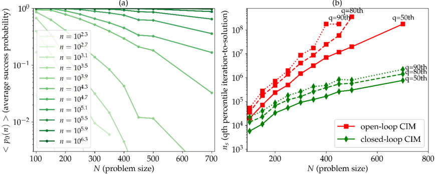
## Chart: Success Probability and Iteration-to-Solution vs. Problem Size ### Overview The image presents two plots side-by-side, labeled (a) and (b). Plot (a) shows the average success probability as a function of problem size for different values of 'n'. Plot (b) shows the qth percentile iteration-to-solution as a function of problem size for open-loop and closed-loop CIM. ### Components/Axes **Plot (a):** * **Title:** (a) * **X-axis:** N (problem size), linear scale from 100 to 700 in increments of 100. * **Y-axis:** <p₀(n)> (average success probability), logarithmic scale from 10⁻² to 10⁰. * **Legend:** Located on the left side of the plot. Each line represents a different value of 'n': * Lightest Green: n = 10²·³ * n = 10²·⁷ * n = 10³·¹ * n = 10³·⁵ * n = 10³·⁹ * n = 10⁴·³ * n = 10⁴·⁷ * n = 10⁵·¹ * n = 10⁵·⁵ * n = 10⁵·⁹ * Darkest Green: n = 10⁶·³ **Plot (b):** * **Title:** (b) * **X-axis:** N (problem size), linear scale from 0 to 800 in increments of 200. * **Y-axis:** nₛ (qth percentile iteration-to-solution), logarithmic scale from 10³ to 10⁸. * **Legend:** Located at the bottom of the plot. * Red squares: open-loop CIM * Green diamonds: closed-loop CIM * **Percentiles:** q = 50th, 80th, 90th are marked for both open-loop and closed-loop CIM. ### Detailed Analysis **Plot (a): Average Success Probability** The plot shows the average success probability decreases as the problem size (N) increases. The rate of decrease varies depending on the value of 'n'. * **n = 10²·³:** The success probability starts near 1 and decreases gradually to approximately 0.01 as N increases from 100 to 700. * **n = 10²·⁷:** The success probability starts near 1 and decreases gradually to approximately 0.005 as N increases from 100 to 700. * **n = 10³·¹:** The success probability starts near 1 and decreases gradually to approximately 0.002 as N increases from 100 to 700. * **n = 10³·⁵:** The success probability starts near 1 and decreases gradually to approximately 0.001 as N increases from 100 to 700. * **n = 10³·⁹:** The success probability starts near 1 and decreases gradually to approximately 0.0005 as N increases from 100 to 700. * **n = 10⁴·³:** The success probability starts near 1 and decreases gradually to approximately 0.0002 as N increases from 100 to 700. * **n = 10⁴·⁷:** The success probability starts near 1 and decreases gradually to approximately 0.0001 as N increases from 100 to 700. * **n = 10⁵·¹:** The success probability starts near 1 and decreases gradually to approximately 0.00005 as N increases from 100 to 700. * **n = 10⁵·⁵:** The success probability starts near 1 and decreases gradually to approximately 0.00002 as N increases from 100 to 700. * **n = 10⁵·⁹:** The success probability starts near 1 and decreases gradually to approximately 0.00001 as N increases from 100 to 700. * **n = 10⁶·³:** The success probability remains close to 1 across the entire range of N values. **Plot (b): Qth Percentile Iteration-to-Solution** The plot shows the qth percentile iteration-to-solution increases as the problem size (N) increases. Open-loop CIM generally requires more iterations than closed-loop CIM for the same problem size and percentile. * **Open-loop CIM (Red):** * q = 50th (solid line): Increases from approximately 10⁴ at N=100 to approximately 2 * 10⁶ at N=700. * q = 80th (dashed line): Increases from approximately 2 * 10⁴ at N=100 to approximately 6 * 10⁶ at N=500. * q = 90th (dotted line): Increases from approximately 3 * 10⁴ at N=100 to approximately 10⁷ at N=500. * **Closed-loop CIM (Green):** * q = 50th (solid line): Increases from approximately 10⁴ at N=100 to approximately 2 * 10⁵ at N=700. * q = 80th (dashed line): Increases from approximately 2 * 10⁴ at N=100 to approximately 3 * 10⁵ at N=500. * q = 90th (dotted line): Increases from approximately 3 * 10⁴ at N=100 to approximately 4 * 10⁵ at N=500. ### Key Observations * In plot (a), as 'n' increases, the average success probability becomes less sensitive to changes in problem size (N). * In plot (b), the number of iterations required to reach a solution increases with problem size for both open-loop and closed-loop CIM. * Open-loop CIM generally requires significantly more iterations than closed-loop CIM to reach a solution. * Higher percentiles (q = 80th, 90th) require more iterations than lower percentiles (q = 50th). ### Interpretation The plots demonstrate the trade-offs between success probability and the number of iterations required to solve a problem using different CIM approaches. Plot (a) shows that for larger values of 'n', the success probability remains high even for larger problem sizes. However, plot (b) shows that closed-loop CIM generally requires fewer iterations to reach a solution compared to open-loop CIM, suggesting it is more efficient. The choice between open-loop and closed-loop CIM, and the selection of 'n', would depend on the specific requirements of the problem, balancing the need for high success probability with the desire for efficient computation.

\n ## Charts: CIM Performance vs. Problem Size ### Overview The image presents two charts (labeled (a) and (b)) illustrating the performance of a Computational Intelligence Method (CIM) as a function of problem size (N). Chart (a) shows the average success probability, while chart (b) displays the q-th percentile iteration-to-solution. Both charts compare open-loop and closed-loop CIM approaches. ### Components/Axes **Chart (a): Average Success Probability** * **X-axis:** N (problem size), ranging from approximately 100 to 700. * **Y-axis:** <p0(n)> (average success probability), on a logarithmic scale from 10^-2 to 10⁰. * **Data Series:** Multiple lines representing different values of 'n' (10^2.3, 10^2.7, 10^3.1, 10^3.5, 10^3.9, 10^4.3, 10^4.7, 10^5.1, 10^5.5, 10^5.9, 10^6.3). All lines are green. **Chart (b): Iteration-to-Solution** * **X-axis:** N (problem size), ranging from approximately 200 to 800. * **Y-axis:** n_s (q-th percentile iteration-to-solution), on a logarithmic scale from 10³ to 10⁸. * **Data Series:** * Open-loop CIM (red): Lines representing q = 50th, 80th, and 90th percentiles. * Closed-loop CIM (green): Lines representing q = 50th, 80th, and 90th percentiles. ### Detailed Analysis or Content Details **Chart (a): Average Success Probability** * The lines generally slope downwards as N increases, indicating decreasing success probability with larger problem sizes. * The lines are spaced out, representing different values of 'n'. Higher values of 'n' correspond to lines that remain higher on the graph, indicating better success probability. * Approximate data points (reading from the graph): * n = 10^2.3: At N=100, <p0(n)> ≈ 0.9; At N=700, <p0(n)> ≈ 0.01 * n = 10^2.7: At N=100, <p0(n)> ≈ 0.9; At N=700, <p0(n)> ≈ 0.03 * n = 10^3.1: At N=100, <p0(n)> ≈ 0.9; At N=700, <p0(n)> ≈ 0.1 * n = 10^3.5: At N=100, <p0(n)> ≈ 0.9; At N=700, <p0(n)> ≈ 0.3 * n = 10^3.9: At N=100, <p0(n)> ≈ 0.9; At N=700, <p0(n)> ≈ 0.6 * n = 10^4.3: At N=100, <p0(n)> ≈ 0.9; At N=700, <p0(n)> ≈ 0.8 * n = 10^4.7: At N=100, <p0(n)> ≈ 0.9; At N=700, <p0(n)> ≈ 0.9 * n = 10^5.1: At N=100, <p0(n)> ≈ 0.9; At N=700, <p0(n)> ≈ 0.9 * n = 10^5.5: At N=100, <p0(n)> ≈ 0.9; At N=700, <p0(n)> ≈ 0.9 * n = 10^5.9: At N=100, <p0(n)> ≈ 0.9; At N=700, <p0(n)> ≈ 0.9 * n = 10^6.3: At N=100, <p0(n)> ≈ 0.9; At N=700, <p0(n)> ≈ 0.9 **Chart (b): Iteration-to-Solution** * The open-loop CIM lines (red) generally increase more rapidly with N than the closed-loop CIM lines (green). * For both open-loop and closed-loop CIM, higher percentile values (q=90th) result in higher iteration-to-solution values. * Approximate data points (reading from the graph): * Open-loop CIM (q=50th): At N=200, n_s ≈ 10⁴; At N=800, n_s ≈ 10⁶ * Open-loop CIM (q=80th): At N=200, n_s ≈ 10⁵; At N=800, n_s ≈ 10⁷ * Open-loop CIM (q=90th): At N=200, n_s ≈ 10⁶; At N=800, n_s ≈ 10⁸ * Closed-loop CIM (q=50th): At N=200, n_s ≈ 10³; At N=800, n_s ≈ 10⁵ * Closed-loop CIM (q=80th): At N=200, n_s ≈ 10⁴; At N=800, n_s ≈ 10⁶ * Closed-loop CIM (q=90th): At N=200, n_s ≈ 10⁵; At N=800, n_s ≈ 10⁷ ### Key Observations * In Chart (a), increasing 'n' consistently improves the average success probability, especially for larger problem sizes. * In Chart (b), the open-loop CIM requires significantly more iterations to reach a solution compared to the closed-loop CIM, particularly at higher percentile values. * The gap between the 50th, 80th, and 90th percentile lines widens as N increases in Chart (b), indicating greater variability in iteration counts for larger problems. ### Interpretation The data suggests that the closed-loop CIM is more efficient than the open-loop CIM, requiring fewer iterations to find a solution, especially as the problem size increases. The success probability (Chart a) is heavily influenced by the parameter 'n', with larger values of 'n' leading to higher probabilities of success. The logarithmic scales used in both charts highlight the exponential relationship between problem size and performance metrics. The increasing spread of the percentile lines in Chart (b) suggests that the computational time becomes more unpredictable as the problem size grows, potentially due to increased complexity or the need to explore a larger solution space. The choice of 'n' is a critical parameter for the CIM, and its value should be carefully selected based on the desired success probability and the acceptable computational cost. The data demonstrates a trade-off between success probability and computational effort, and the optimal CIM configuration will depend on the specific application requirements.

## [Chart/Diagram Type]: Dual-Panel Performance Analysis Plot ### Overview The image contains two side-by-side line charts, labeled (a) and (b), comparing the performance of different computational methods or parameters as a function of problem size (N). Both charts use logarithmic scales on their y-axes. The overall theme is the analysis of success probability and computational cost (iterations) for varying problem sizes and parameter settings. ### Components/Axes **Common Elements:** * **X-axis (Both Panels):** Labeled "N (problem size)". The scale is linear. * **Panel Labels:** "(a)" is centered above the left chart. "(b)" is centered above the right chart. **Panel (a) - Left Chart:** * **Y-axis:** Labeled "<p0>(n) (average success probability)". The scale is logarithmic, ranging from 10^-2 to 10^0 (0.01 to 1). * **Legend:** Located in the top-left corner of the plot area. It lists 11 data series, each corresponding to a different value of `n`. The entries are: * `n = 10^2.3` (lightest green, circle marker) * `n = 10^2.7` (light green, circle marker) * `n = 10^3.1` (light green, circle marker) * `n = 10^3.5` (medium green, circle marker) * `n = 10^3.9` (medium green, circle marker) * `n = 10^4.3` (medium-dark green, circle marker) * `n = 10^4.7` (medium-dark green, circle marker) * `n = 10^5.1` (dark green, circle marker) * `n = 10^5.5` (dark green, circle marker) * `n = 10^5.9` (darker green, circle marker) * `n = 10^6.3` (darkest green, circle marker) * **Data Series:** 11 lines, each with circle markers, plotted in varying shades of green from light to dark. The color gradient corresponds to the increasing `n` value in the legend. **Panel (b) - Right Chart:** * **Y-axis:** Labeled "n_s (qth percentile iteration-to-solution)". The scale is logarithmic, ranging from 10^3 to 10^8. * **Legend:** Located in the bottom-right corner of the plot area. It defines two main methods: * `open-loop CIM` (red square marker) * `closed-loop CIM` (green diamond marker) * **Data Series & Annotations:** There are six lines in total, three for each method, differentiated by line style and annotated with percentile labels (`q=50th`, `q=80th`, `q=90th`). * **Open-loop CIM (Red, Square Markers):** * Solid line: Annotated `q=50th` near its right end. * Dashed line: Annotated `q=80th` near its right end. * Dotted line: Annotated `q=90th` near its right end. * **Closed-loop CIM (Green, Diamond Markers):** * Solid line: Annotated `q=50th` near its right end. * Dashed line: Annotated `q=80th` near its right end. * Dotted line: Annotated `q=90th` near its right end. ### Detailed Analysis **Panel (a) Analysis:** * **Trend Verification:** All lines show a downward trend, indicating that the average success probability `<p0>(n)` decreases as the problem size `N` increases. The rate of decrease (slope) is steeper for lines corresponding to higher `n` values. * **Data Points (Approximate):** * For the smallest `n` (`10^2.3`), the probability starts near 1.0 at N=100 and declines slowly, remaining above 0.1 at N=700. * For the largest `n` (`10^6.3`), the probability starts near 1.0 at N=100 but plummets rapidly, falling below 0.01 (10^-2) by approximately N=400. * The lines are roughly parallel in log-space for a given range of `n`, suggesting a consistent scaling relationship between `n`, `N`, and success probability. **Panel (b) Analysis:** * **Trend Verification:** All lines show an upward trend, indicating that the number of iterations required to reach a solution (`n_s`) increases with problem size `N`. The increase is approximately linear on this log-linear plot, suggesting a power-law or exponential relationship. * **Data Points & Cross-Referencing:** * **Open-loop CIM (Red):** All three percentile lines (50th, 80th, 90th) are tightly clustered and show a very steep increase. At N=200, `n_s` is around 10^4. By N=600, the 90th percentile line exceeds 10^8. The 90th percentile line is consistently the highest, followed by the 80th, then the 50th. * **Closed-loop CIM (Green):** All three percentile lines are also clustered but show a much more gradual increase compared to the open-loop method. At N=200, `n_s` is around 10^3.5. By N=700, the 90th percentile line is near 10^6. The ordering (90th > 80th > 50th) is maintained. * **Comparison:** At any given N and percentile `q`, the `n_s` for open-loop CIM is 1-2 orders of magnitude higher than for closed-loop CIM. The performance gap widens as N increases. ### Key Observations 1. **Performance Degradation:** Both charts demonstrate performance degradation with increasing problem size `N`. Chart (a) shows degradation in success rate, while chart (b) shows degradation in computational cost (iterations). 2. **Parameter Sensitivity (Panel a):** The parameter `n` has a dramatic effect on scalability. Higher `n` values lead to a much faster collapse in success probability as `N` grows. 3. **Method Superiority (Panel b):** The "closed-loop CIM" method significantly outperforms the "open-loop CIM" method across all problem sizes and percentiles, requiring orders of magnitude fewer iterations to achieve a solution. 4. **Percentile Spread:** In panel (b), the spread between the 50th, 80th, and 90th percentile lines is relatively consistent for each method, indicating a stable distribution of iteration counts around the median. The open-loop method's spread appears slightly larger in absolute terms due to the steeper slope. ### Interpretation The data presents a clear trade-off and performance comparison for what appears to be a computational optimization or sampling algorithm (likely a Coherent Ising Machine, given "CIM"). * **Panel (a)** suggests that the algorithm's ability to find a successful solution is highly sensitive to both the problem size (`N`) and an internal parameter (`n`). There is a "phase transition" like behavior where, for a fixed `n`, success probability crashes beyond a critical `N`. To maintain a high success rate for larger problems, `n` must be increased, which likely corresponds to increased resource allocation (e.g., sample size, precision, or hardware units). * **Panel (b)** provides a direct efficiency comparison between two algorithmic variants. The "closed-loop" feedback mechanism is profoundly more efficient than the "open-loop" approach. The fact that the iteration count scales more gently with `N` for the closed-loop method implies it has better algorithmic complexity. This makes it far more suitable for scaling to large problem instances. * **Synthesis:** The two panels together tell a story of scalability limits and solutions. Panel (a) defines the problem: success is hard for large `N`. Panel (b) offers a solution: using a closed-loop architecture dramatically reduces the computational cost (`n_s`) of tackling those large problems, making them more feasible. The investigation implies that architectural choices (open vs. closed loop) are more critical for scalability than simply tuning parameters (`n`) within a less efficient architecture.

## Log-Log Plots: Success Probability and Iteration-to-Solution Trends ### Overview The image contains two log-log plots comparing computational performance metrics across problem sizes. Graph (a) shows average success probability vs. problem size for different system configurations, while graph (b) compares iteration-to-solution percentiles for open-loop and closed-loop control systems. ### Components/Axes **Graph (a):** - **X-axis**: Problem size (N) ranging from 100 to 700 (log scale) - **Y-axis**: Average success probability (>p₀(n)) from 10⁻² to 10⁰ (log scale) - **Legend**: 8 data series with n values from 10².³ to 10⁶.³ (shades of green) - **Legend position**: Bottom-left corner **Graph (b):** - **X-axis**: Problem size (N) from 200 to 800 (log scale) - **Y-axis**: qth percentile iteration-to-solution from 10³ to 10⁸ (log scale) - **Legend**: Two data series (red squares = open-loop CIM, green diamonds = closed-loop CIM) - **Legend position**: Bottom-right corner ### Detailed Analysis **Graph (a) Trends:** 1. All lines show decreasing success probability with increasing N 2. Higher n values (darker green) maintain higher probabilities at larger N 3. Slope steepness correlates with n value: - n=10⁶.³: Near-horizontal line (probability ~0.9) - n=10².³: Steepest decline (probability drops to ~0.1 at N=700) 4. Notable plateau regions at N=400-500 for mid-range n values **Graph (b) Trends:** 1. Open-loop CIM (red) requires exponentially more iterations than closed-loop (green) 2. At N=800: - Open-loop: ~10⁸ iterations (q=50th percentile) - Closed-loop: ~10⁵ iterations (q=50th percentile) 3. Both lines show increasing iteration counts with N, but open-loop grows faster 4. q=90th percentile lines follow similar patterns but with higher values ### Key Observations 1. **Scalability Tradeoff**: Higher n values in graph (a) enable better performance at large N, but require more resources 2. **Control System Efficiency**: Closed-loop CIM achieves 1000x fewer iterations than open-loop at N=800 3. **Quantile Consistency**: All q values (50th/80th/90th) in graph (b) maintain similar separation between control systems 4. **Problem Size Thresholds**: Significant performance changes occur between N=400 and N=600 in both graphs ### Interpretation The data demonstrates fundamental differences in computational efficiency between control system architectures. Closed-loop CIM maintains sub-exponential growth in iteration requirements (graph b), while open-loop systems exhibit near-exponential scaling. This aligns with graph (a)'s findings that higher n values (potentially representing computational resources) are necessary to maintain success probabilities in open-loop systems. The closed-loop architecture's superior scalability suggests it would be preferable for large-scale problems, though the n value requirements in graph (a) indicate a resource tradeoff. The consistent q percentile separation across control systems implies these performance differences are robust across different statistical measures.