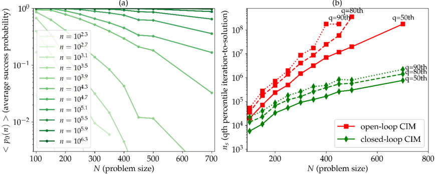
## [Chart/Diagram Type]: Dual-Panel Performance Analysis Plot ### Overview The image contains two side-by-side line charts, labeled (a) and (b), comparing the performance of different computational methods or parameters as a function of problem size (N). Both charts use logarithmic scales on their y-axes. The overall theme is the analysis of success probability and computational cost (iterations) for varying problem sizes and parameter settings. ### Components/Axes **Common Elements:** * **X-axis (Both Panels):** Labeled "N (problem size)". The scale is linear. * **Panel Labels:** "(a)" is centered above the left chart. "(b)" is centered above the right chart. **Panel (a) - Left Chart:** * **Y-axis:** Labeled "<p0>(n) (average success probability)". The scale is logarithmic, ranging from 10^-2 to 10^0 (0.01 to 1). * **Legend:** Located in the top-left corner of the plot area. It lists 11 data series, each corresponding to a different value of `n`. The entries are: * `n = 10^2.3` (lightest green, circle marker) * `n = 10^2.7` (light green, circle marker) * `n = 10^3.1` (light green, circle marker) * `n = 10^3.5` (medium green, circle marker) * `n = 10^3.9` (medium green, circle marker) * `n = 10^4.3` (medium-dark green, circle marker) * `n = 10^4.7` (medium-dark green, circle marker) * `n = 10^5.1` (dark green, circle marker) * `n = 10^5.5` (dark green, circle marker) * `n = 10^5.9` (darker green, circle marker) * `n = 10^6.3` (darkest green, circle marker) * **Data Series:** 11 lines, each with circle markers, plotted in varying shades of green from light to dark. The color gradient corresponds to the increasing `n` value in the legend. **Panel (b) - Right Chart:** * **Y-axis:** Labeled "n_s (qth percentile iteration-to-solution)". The scale is logarithmic, ranging from 10^3 to 10^8. * **Legend:** Located in the bottom-right corner of the plot area. It defines two main methods: * `open-loop CIM` (red square marker) * `closed-loop CIM` (green diamond marker) * **Data Series & Annotations:** There are six lines in total, three for each method, differentiated by line style and annotated with percentile labels (`q=50th`, `q=80th`, `q=90th`). * **Open-loop CIM (Red, Square Markers):** * Solid line: Annotated `q=50th` near its right end. * Dashed line: Annotated `q=80th` near its right end. * Dotted line: Annotated `q=90th` near its right end. * **Closed-loop CIM (Green, Diamond Markers):** * Solid line: Annotated `q=50th` near its right end. * Dashed line: Annotated `q=80th` near its right end. * Dotted line: Annotated `q=90th` near its right end. ### Detailed Analysis **Panel (a) Analysis:** * **Trend Verification:** All lines show a downward trend, indicating that the average success probability `<p0>(n)` decreases as the problem size `N` increases. The rate of decrease (slope) is steeper for lines corresponding to higher `n` values. * **Data Points (Approximate):** * For the smallest `n` (`10^2.3`), the probability starts near 1.0 at N=100 and declines slowly, remaining above 0.1 at N=700. * For the largest `n` (`10^6.3`), the probability starts near 1.0 at N=100 but plummets rapidly, falling below 0.01 (10^-2) by approximately N=400. * The lines are roughly parallel in log-space for a given range of `n`, suggesting a consistent scaling relationship between `n`, `N`, and success probability. **Panel (b) Analysis:** * **Trend Verification:** All lines show an upward trend, indicating that the number of iterations required to reach a solution (`n_s`) increases with problem size `N`. The increase is approximately linear on this log-linear plot, suggesting a power-law or exponential relationship. * **Data Points & Cross-Referencing:** * **Open-loop CIM (Red):** All three percentile lines (50th, 80th, 90th) are tightly clustered and show a very steep increase. At N=200, `n_s` is around 10^4. By N=600, the 90th percentile line exceeds 10^8. The 90th percentile line is consistently the highest, followed by the 80th, then the 50th. * **Closed-loop CIM (Green):** All three percentile lines are also clustered but show a much more gradual increase compared to the open-loop method. At N=200, `n_s` is around 10^3.5. By N=700, the 90th percentile line is near 10^6. The ordering (90th > 80th > 50th) is maintained. * **Comparison:** At any given N and percentile `q`, the `n_s` for open-loop CIM is 1-2 orders of magnitude higher than for closed-loop CIM. The performance gap widens as N increases. ### Key Observations 1. **Performance Degradation:** Both charts demonstrate performance degradation with increasing problem size `N`. Chart (a) shows degradation in success rate, while chart (b) shows degradation in computational cost (iterations). 2. **Parameter Sensitivity (Panel a):** The parameter `n` has a dramatic effect on scalability. Higher `n` values lead to a much faster collapse in success probability as `N` grows. 3. **Method Superiority (Panel b):** The "closed-loop CIM" method significantly outperforms the "open-loop CIM" method across all problem sizes and percentiles, requiring orders of magnitude fewer iterations to achieve a solution. 4. **Percentile Spread:** In panel (b), the spread between the 50th, 80th, and 90th percentile lines is relatively consistent for each method, indicating a stable distribution of iteration counts around the median. The open-loop method's spread appears slightly larger in absolute terms due to the steeper slope. ### Interpretation The data presents a clear trade-off and performance comparison for what appears to be a computational optimization or sampling algorithm (likely a Coherent Ising Machine, given "CIM"). * **Panel (a)** suggests that the algorithm's ability to find a successful solution is highly sensitive to both the problem size (`N`) and an internal parameter (`n`). There is a "phase transition" like behavior where, for a fixed `n`, success probability crashes beyond a critical `N`. To maintain a high success rate for larger problems, `n` must be increased, which likely corresponds to increased resource allocation (e.g., sample size, precision, or hardware units). * **Panel (b)** provides a direct efficiency comparison between two algorithmic variants. The "closed-loop" feedback mechanism is profoundly more efficient than the "open-loop" approach. The fact that the iteration count scales more gently with `N` for the closed-loop method implies it has better algorithmic complexity. This makes it far more suitable for scaling to large problem instances. * **Synthesis:** The two panels together tell a story of scalability limits and solutions. Panel (a) defines the problem: success is hard for large `N`. Panel (b) offers a solution: using a closed-loop architecture dramatically reduces the computational cost (`n_s`) of tackling those large problems, making them more feasible. The investigation implies that architectural choices (open vs. closed loop) are more critical for scalability than simply tuning parameters (`n`) within a less efficient architecture.