## Bar Chart: Subtractor: Time vs Core count ### Overview The image is a bar chart that displays the relationship between the time taken (in milliseconds) and the core count for a "Subtractor" operation. The x-axis represents the core count, ranging from 1 to 47. The y-axis represents the time in milliseconds, ranging from 0 to 6000. The chart shows a general trend of decreasing time with an increasing number of cores, with a steep drop initially, followed by a more gradual decrease. ### Components/Axes * **Title:** Subtractor: Time vs Core count * **X-axis:** * Label: Core count * Scale: 1 to 47, incrementing by 2 (1, 3, 5, 7, ..., 47) * **Y-axis:** * Label: Time (ms) * Scale: 0 to 6000, incrementing by 1000 (0, 1000, 2000, 3000, 4000, 5000, 6000) * **Data:** Blue bars representing the time taken for each core count. ### Detailed Analysis Here's a breakdown of the approximate time values for different core counts: * **1 Core:** Approximately 5050 ms * **3 Cores:** Approximately 4600 ms * **5 Cores:** Approximately 2450 ms * **7 Cores:** Approximately 1750 ms * **9 Cores:** Approximately 1700 ms * **11 Cores:** Approximately 1350 ms * **13 Cores:** Approximately 1000 ms * **15 Cores:** Approximately 950 ms * **17 Cores:** Approximately 800 ms * **19 Cores:** Approximately 750 ms * **21 Cores:** Approximately 700 ms * **23 Cores:** Approximately 700 ms * **25 Cores:** Approximately 650 ms * **27 Cores:** Approximately 650 ms * **29 Cores:** Approximately 600 ms * **31 Cores:** Approximately 600 ms * **33 Cores:** Approximately 650 ms * **35 Cores:** Approximately 650 ms * **37 Cores:** Approximately 650 ms * **39 Cores:** Approximately 650 ms * **41 Cores:** Approximately 700 ms * **43 Cores:** Approximately 700 ms * **45 Cores:** Approximately 700 ms * **47 Cores:** Approximately 700 ms **Trend:** The time decreases rapidly from 1 core to approximately 11 cores. After that, the decrease is much slower, and the time seems to plateau around 700 ms. ### Key Observations * The most significant reduction in time occurs when increasing the core count from 1 to around 11. * Beyond 11 cores, the benefit of adding more cores diminishes significantly. * The time appears to stabilize around 700 ms for core counts greater than 35. ### Interpretation The data suggests that increasing the number of cores for the "Subtractor" operation initially leads to a substantial reduction in processing time, indicating effective parallelization. However, after a certain point (around 11 cores), the gains from adding more cores become marginal. This could be due to factors such as communication overhead between cores, limitations in the algorithm's parallelizability, or other bottlenecks in the system. The plateauing of time around 700 ms suggests that there might be a fundamental limit to how fast the operation can be performed, regardless of the number of cores used.

\n ## Bar Chart: Subtractor - Time vs Core count ### Overview The image presents a bar chart illustrating the relationship between the time taken (in milliseconds) for a "Subtractor" operation and the number of cores used. The chart displays a decreasing trend in execution time as the number of cores increases, with a rapid initial decrease followed by a leveling off. ### Components/Axes * **Title:** Subtractor: Time vs Core count * **X-axis:** Core count. Markers are present at integer values from 1 to 47. * **Y-axis:** Time (ms). Scale ranges from 0 to 6000 milliseconds. * **Data Series:** A single series of bars representing the time taken for each core count. * **Bar Color:** Light blue. ### Detailed Analysis The chart shows a significant decrease in execution time as the core count increases from 1 to approximately 11. Beyond 11 cores, the reduction in execution time becomes much less pronounced, eventually leveling off around 600-800 ms. Here's a breakdown of approximate values, reading from the chart: * **1 Core:** ~4900 ms * **3 Cores:** ~2300 ms * **5 Cores:** ~1700 ms * **7 Cores:** ~1300 ms * **9 Cores:** ~1100 ms * **11 Cores:** ~900 ms * **13 Cores:** ~800 ms * **15 Cores:** ~750 ms * **17 Cores:** ~700 ms * **19 Cores:** ~650 ms * **21 Cores:** ~600 ms * **23 Cores:** ~580 ms * **25 Cores:** ~560 ms * **27 Cores:** ~540 ms * **29 Cores:** ~530 ms * **31 Cores:** ~520 ms * **33 Cores:** ~510 ms * **35 Cores:** ~500 ms * **37 Cores:** ~490 ms * **39 Cores:** ~480 ms * **41 Cores:** ~470 ms * **43 Cores:** ~460 ms * **45 Cores:** ~450 ms * **47 Cores:** ~440 ms The trend is a steep decline from 1 to 11 cores, followed by diminishing returns as more cores are added. ### Key Observations * The most significant performance gains are achieved with a relatively small number of cores (1-11). * Adding cores beyond 11 yields progressively smaller improvements in execution time. * The execution time appears to converge towards a minimum value of approximately 440-500 ms as the core count increases. ### Interpretation The data suggests that the "Subtractor" operation benefits from parallelization, as evidenced by the decreasing execution time with increasing core count. However, the benefits of parallelization diminish beyond a certain point, indicating that the operation may be limited by factors other than the number of available cores (e.g., memory bandwidth, algorithm complexity, or inherent sequential dependencies). The leveling off of the curve suggests that the operation has reached a point where adding more cores does not significantly reduce the time required to complete the task. This could be due to Amdahl's Law, where a portion of the task remains inherently sequential and cannot be parallelized. The initial steep decline indicates a highly parallelizable component of the operation. The chart provides valuable insight into the scalability of the "Subtractor" operation and can inform decisions about resource allocation and optimization strategies.

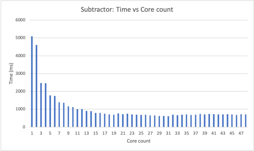
## Bar Chart: Subtractor Performance vs. Core Count ### Overview The image displays a vertical bar chart titled "Subtractor: Time vs Core count." It illustrates the relationship between the number of processing cores used (x-axis) and the execution time in milliseconds (y-axis) for a computational task labeled "Subtractor." The chart demonstrates a clear performance scaling trend. ### Components/Axes * **Chart Title:** "Subtractor: Time vs Core count" (centered at the top). * **Y-Axis:** * **Label:** "Time (ms)" (rotated vertically on the left side). * **Scale:** Linear scale from 0 to 6000. * **Major Gridlines & Tick Marks:** At 0, 1000, 2000, 3000, 4000, 5000, and 6000 ms. * **X-Axis:** * **Label:** "Core count" (centered at the bottom). * **Scale:** Discrete, linear scale representing core counts. * **Tick Marks & Labels:** Labeled at every odd number from 1 to 47 (1, 3, 5, ..., 47). Bars exist for every integer core count from 1 to 48, but only odd numbers are labeled. * **Data Series:** A single series represented by blue vertical bars. Each bar's height corresponds to the execution time for a specific core count. * **Legend:** Not present. The chart contains only one data series. ### Detailed Analysis **Trend Verification:** The data series shows a strong, inverse relationship. The line formed by the bar tops slopes steeply downward from left to right initially, then flattens into a near-horizontal plateau. This indicates that execution time decreases rapidly as cores are added from 1 to approximately 15, after which further increases in core count yield minimal time reduction. **Spatial Grounding & Approximate Data Points:** * **Core Count 1:** The tallest bar, located at the far left. Its top aligns just above the 5000 ms gridline. **Approximate Value: 5050 ms.** * **Core Count 2:** The second bar. Its top is between the 4000 and 5000 ms lines, closer to 5000. **Approximate Value: 4600 ms.** * **Core Count 3:** The third bar. Its top is roughly midway between 2000 and 3000 ms. **Approximate Value: 2500 ms.** * **Core Count 4:** The fourth bar. Its height is very similar to core count 3. **Approximate Value: 2450 ms.** * **Core Count 5:** The fifth bar. Its top is below the 2000 ms line. **Approximate Value: 1750 ms.** * **Core Count 7:** The seventh bar. **Approximate Value: 1350 ms.** * **Core Count 9:** The ninth bar. **Approximate Value: 1100 ms.** * **Core Count 11:** The eleventh bar. **Approximate Value: 1000 ms.** * **Core Count 13:** The thirteenth bar. **Approximate Value: 900 ms.** * **Core Count 15:** The fifteenth bar. **Approximate Value: 800 ms.** * **Core Count 17 to 48:** From approximately core count 17 onward, the bar heights stabilize. They fluctuate slightly but remain consistently in the range of **600 ms to 800 ms**. The lowest point appears around core counts 29-31, near **600 ms**. The final bar (core count 48) is approximately **750 ms**. ### Key Observations 1. **Diminishing Returns:** The most significant performance gain occurs when moving from 1 to 2 cores (a ~450 ms reduction) and from 2 to 3 cores (a dramatic ~2100 ms reduction). Gains become progressively smaller after ~15 cores. 2. **Performance Plateau:** After approximately 15-20 cores, adding more cores does not result in a meaningful decrease in execution time. The time stabilizes in the 600-800 ms range. 3. **Initial Anomaly:** The time for 2 cores is only slightly less than for 1 core, while the drop to 3 cores is massive. This suggests a potential overhead or non-parallelizable component that is efficiently overcome only with 3 or more cores. 4. **Consistency:** The plateau region shows very low variance, indicating stable performance scaling behavior at higher core counts. ### Interpretation This chart visualizes the **Amdahl's Law** or **Gustafson's Law** principle in parallel computing. The "Subtractor" task has a portion that can be parallelized (the steep decline) and a portion that is serial or has fixed overhead (the plateau). * **What the data suggests:** The task benefits greatly from parallelization up to a point. The optimal resource allocation for this specific task appears to be around 15-20 cores. Using more than 20 cores is inefficient, as it consumes additional computational resources without reducing runtime, indicating the parallelizable portion of the work has been fully saturated. * **How elements relate:** The x-axis (Core count) is the independent variable representing resource投入. The y-axis (Time) is the dependent variable representing performance. The inverse curve is the direct result of applying more resources to the parallelizable workload. * **Notable outliers:** The relatively small improvement from 1 to 2 cores compared to the leap from 2 to 3 is the most notable anomaly. This could indicate a specific implementation detail, such as a two-threaded process that still contends for a shared resource, which is alleviated when a third thread is introduced. * **Practical Implication:** For a system engineer, this chart provides clear guidance: allocating more than ~20 cores to this specific "Subtractor" process is wasteful. The ideal configuration balances performance (near 600 ms) with resource cost.

## Bar Chart: Subtractor: Time vs Core count ### Overview The bar chart displays the time taken by a subtractor in milliseconds (ms) as a function of the core count. The x-axis represents the core count, which ranges from 1 to 47, while the y-axis represents the time taken in milliseconds, ranging from 0 to 6000 ms. ### Components/Axes - **Title**: Subtractor: Time vs Core count - **X-axis**: Core count, ranging from 1 to 47 - **Y-axis**: Time (ms), ranging from 0 to 6000 ms - **Legend**: No legend is present in the image ### Detailed Analysis or ### Content Details The chart shows a clear trend where the time taken by the subtractor decreases as the core count increases. The highest time taken is approximately 5000 ms at a core count of 1, and the time taken decreases gradually as the core count increases. The time taken at a core count of 47 is approximately 1000 ms. ### Key Observations - The time taken by the subtractor decreases as the core count increases. - The highest time taken is at a core count of 1. - The time taken at a core count of 47 is significantly lower than at a core count of 1. ### Interpretation The data suggests that the subtractor's performance improves as the number of cores increases. This is because the subtractor can utilize multiple cores to perform the subtraction operation in parallel, reducing the overall time taken. The trend is consistent across the entire range of core counts, indicating that the subtractor is designed to take advantage of multiple cores to improve performance.

## Bar Chart: Subtractor: Time vs Core count ### Overview The chart visualizes the relationship between computational core count and execution time (in milliseconds) for a "Subtractor" algorithm. Execution time decreases as core count increases, with a sharp decline at lower core counts followed by a plateau at higher counts. ### Components/Axes - **Title**: "Subtractor: Time vs Core count" - **X-axis (Core count)**: Discrete values from 1 to 47, labeled at intervals of 2 (1, 3, 5, ..., 47). - **Y-axis (Time, ms)**: Continuous scale from 0 to 6000 ms, with gridlines at 1000 ms intervals. - **Bars**: Blue vertical bars representing execution time for each core count. No explicit legend is present. ### Detailed Analysis - **Core 1**: Execution time peaks at ~5000 ms. - **Core 3**: Time drops to ~4500 ms. - **Cores 5–11**: Gradual decline, with times ranging from ~1800 ms (core 5) to ~1000 ms (core 11). - **Cores 13–47**: Time stabilizes between ~600 ms and ~700 ms, with minimal variation. - **Trend**: Execution time decreases non-linearly at lower core counts, then plateaus after ~11 cores. ### Key Observations 1. **Diminishing Returns**: The most significant time reduction occurs between 1 and 11 cores. Beyond this, additional cores yield negligible improvements (~600–700 ms). 2. **Outlier**: Core 1 exhibits the highest execution time (~5000 ms), suggesting single-core inefficiency. 3. **Stability**: Cores 31–47 show consistent performance (~600–700 ms), indicating saturation of parallel processing benefits. ### Interpretation The data demonstrates that increasing core count improves performance up to a critical threshold (~11 cores), after which further cores provide little benefit. This suggests: - **Parallelization Limits**: The algorithm may not scale efficiently beyond 11 cores due to overhead (e.g., synchronization, memory contention). - **Hardware Constraints**: Diminishing returns could reflect physical or architectural limits in core coordination. - **Optimization Opportunity**: Refactoring the algorithm to better utilize >11 cores might reduce the plateau. The chart underscores the importance of balancing core count with algorithmic efficiency in high-performance computing.