## Histograms: Reward Distributions of Two Algorithms
### Overview
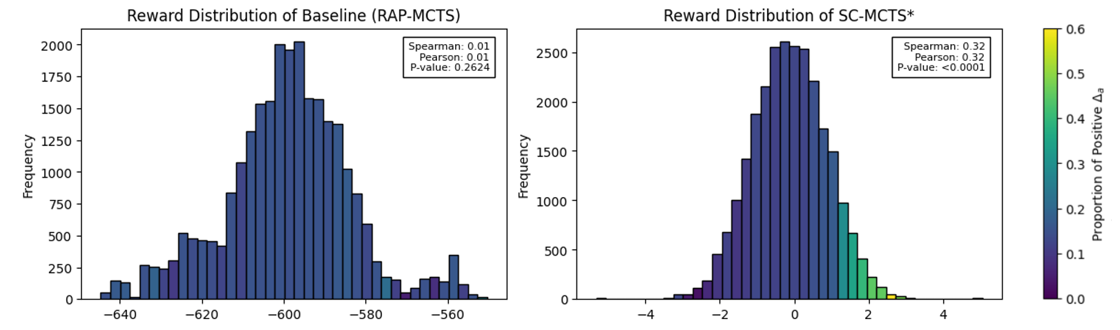
The image displays two side-by-side histograms comparing the reward distributions of two different algorithms or methods. The left histogram represents a "Baseline" method labeled "RAP-MCTS," and the right histogram represents a method labeled "SC-MCTS*." A shared color bar on the far right provides a third dimension of data, indicating the "Proportion of Positive Δa" for the histogram bars.
### Components/Axes
**Left Histogram: "Reward Distribution of Baseline (RAP-MCTS)"**
* **X-axis:** Label is not explicitly written, but the tick marks and context indicate it represents "Reward" values. The scale ranges from approximately -650 to -550, with major tick marks at -640, -620, -600, -580, and -560.
* **Y-axis:** Label is "Frequency." The scale ranges from 0 to 2000, with major tick marks at 0, 250, 500, 750, 1000, 1250, 1500, 1750, and 2000.
* **Text Box (Top-Right Corner):** Contains statistical correlation data.
* `Spearman: 0.01`
* `Pearson: 0.01`
* `P-value: 0.2624`
**Right Histogram: "Reward Distribution of SC-MCTS*"**
* **X-axis:** Label is not explicitly written, but represents "Reward" values. The scale ranges from approximately -5 to 5, with major tick marks at -4, -2, 0, 2, and 4.
* **Y-axis:** Label is "Frequency." The scale ranges from 0 to 2500, with major tick marks at 0, 500, 1000, 1500, 2000, and 2500.
* **Text Box (Top-Right Corner):** Contains statistical correlation data.
* `Spearman: 0.32`
* `Pearson: 0.32`
* `P-value: <0.0001`
**Shared Color Bar (Far Right)**
* **Label:** "Proportion of Positive Δa"
* **Scale:** Ranges from 0.0 to 0.6, with major tick marks at 0.0, 0.1, 0.2, 0.3, 0.4, 0.5, and 0.6.
* **Color Gradient:** A vertical gradient from dark purple (0.0) through blue and green to bright yellow (0.6). This color is applied to the bars in both histograms.
### Detailed Analysis
**Left Histogram (RAP-MCTS):**
* **Trend:** The distribution is roughly unimodal and approximately normal (bell-shaped), centered around a reward value of -600.
* **Data Points:** The highest frequency bars (peak) are located between -605 and -595, reaching a frequency of approximately 2000. The distribution has a visible spread, with significant frequencies from about -630 to -570. There are smaller, secondary clusters of bars around -630 and -560.
* **Color Coding:** The bars are predominantly dark blue/purple, indicating a low "Proportion of Positive Δa" (close to 0.0 to 0.1) across most of the reward range. A few bars on the far right tail (around -560) show a slightly lighter blue/green hue, suggesting a marginally higher proportion.
**Right Histogram (SC-MCTS*):**
* **Trend:** The distribution is unimodal and approximately normal, centered very close to a reward value of 0. It appears slightly right-skewed.
* **Data Points:** The peak frequency is located between -0.5 and 0.5, reaching a frequency of approximately 2600. The bulk of the data lies between -2 and 2. The distribution has a longer, more populated right tail extending to +4 compared to its left tail.
* **Color Coding:** This histogram shows a clear color gradient. Bars on the left side (negative rewards, e.g., -2 to 0) are dark purple/blue (low proportion). As rewards increase towards 0 and into positive values, the bars transition through teal and green. The bars on the far right (rewards > 2) are bright green to yellow, indicating a high "Proportion of Positive Δa" (approaching 0.5 to 0.6).
### Key Observations
1. **Dramatic Shift in Reward Scale:** The baseline (RAP-MCTS) operates in a deeply negative reward space (centered at -600), while SC-MCTS* operates around zero. This suggests SC-MCTS* achieves significantly higher raw reward values.
2. **Correlation with Δa:** The color coding reveals a strong relationship between reward value and the "Proportion of Positive Δa" for SC-MCTS*, which is absent in the baseline. Higher rewards in SC-MCTS* are strongly associated with a higher proportion of positive Δa.
3. **Statistical Significance:** The text boxes show that the correlation (Spearman/Pearson = 0.32) in SC-MCTS* is statistically significant (p < 0.0001), while the near-zero correlation in the baseline is not (p = 0.2624).
4. **Distribution Shape:** Both distributions are roughly normal, but the SC-MCTS* distribution is tighter around its mean (0) relative to its scale and has a more pronounced right tail.
### Interpretation
This visualization demonstrates the superior performance and a key mechanistic insight of the SC-MCTS* algorithm compared to the RAP-MCTS baseline.
* **Performance Improvement:** The shift from a reward distribution centered at -600 to one centered at 0 indicates that SC-MCTS* is far more effective at the task, achieving rewards that are orders of magnitude higher (less negative/more positive).
* **Mechanistic Insight:** The color gradient in the SC-MCTS* plot is the critical finding. It shows that the algorithm's success (higher reward) is directly linked to a higher "Proportion of Positive Δa." Δa likely represents a change in an action or advantage estimate. Therefore, the data suggests that SC-MCTS*'s improvement stems from its ability to generate and select actions that lead to positive changes (Δa), and this ability is quantitatively correlated with the final reward outcome. The baseline shows no such relationship, implying its search process does not effectively leverage this signal.
* **Conclusion:** SC-MCTS* is not only better in outcome but also operates on a more effective and interpretable principle, where progress (positive Δa) is directly tied to success (higher reward). The statistically significant correlation provides strong evidence for this relationship.