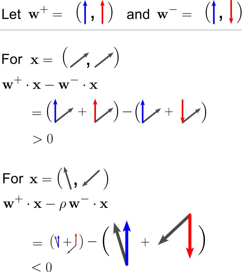
## [Mathematical Diagram]: Vector Dot Product Illustration for Weighted Classification ### Overview The image is a mathematical illustration demonstrating vector dot product calculations for two input vectors \( \boldsymbol{\mathbf{x}} \), using two weight vectors \( \boldsymbol{\mathbf{w}}^+ \) and \( \boldsymbol{\mathbf{w}}^- \). It includes text, vector symbols (arrows), and algebraic expressions to show how different input patterns interact with the weight vectors. ### Components/Elements - **Text Elements**: - Top: *"Let \( \boldsymbol{\mathbf{w}}^+ = (\uparrow, \uparrow) \) and \( \boldsymbol{\mathbf{w}}^- = (\uparrow, \downarrow) \)"* (defines two weight vectors). - First case: *"For \( \boldsymbol{\mathbf{x}} = (\nearrow, \nearrow) \)"* (input vector with two right-up arrows), followed by the expression \( \boldsymbol{\mathbf{w}}^+ \cdot \boldsymbol{\mathbf{x}} - \boldsymbol{\mathbf{w}}^- \cdot \boldsymbol{\mathbf{x}} \), expanded form, and result \( > 0 \). - Second case: *"For \( \boldsymbol{\mathbf{x}} = (\nwarrow, \searrow) \)"* (input vector with left-up and right-down arrows), followed by the expression \( \boldsymbol{\mathbf{w}}^+ \cdot \boldsymbol{\mathbf{x}} - \rho \boldsymbol{\mathbf{w}}^- \cdot \boldsymbol{\mathbf{x}} \) (with scalar \( \rho \)), expanded form, and result \( < 0 \). - **Vector Symbols**: - \( \boldsymbol{\mathbf{w}}^+ \): Two upward arrows (blue and red, representing components). - \( \boldsymbol{\mathbf{w}}^- \): One upward (blue) and one downward (red) arrow. - \( \boldsymbol{\mathbf{x}} \) (first case): Two right-up arrows (gray). - \( \boldsymbol{\mathbf{x}} \) (second case): One left-up (gray) and one right-down (gray) arrow. - Dot product illustrations: Arrows showing the dot product (e.g., \( \uparrow \cdot \nearrow \) as a blue arrow with a gray arrow). ### Detailed Analysis #### Case 1: \( \boldsymbol{\mathbf{x}} = (\nearrow, \nearrow) \) - **Expression**: \( \boldsymbol{\mathbf{w}}^+ \cdot \boldsymbol{\mathbf{x}} - \boldsymbol{\mathbf{w}}^- \cdot \boldsymbol{\mathbf{x}} \) - **Expanded Form**: \( (\uparrow \cdot \nearrow + \uparrow \cdot \nearrow) - (\uparrow \cdot \nearrow + \downarrow \cdot \nearrow) \) - **Simplification**: \( (\uparrow \cdot \nearrow - \downarrow \cdot \nearrow) + (\uparrow \cdot \nearrow - \uparrow \cdot \nearrow) = (\uparrow - \downarrow) \cdot \nearrow \) - **Result**: \( > 0 \) (since \( \uparrow \) and \( \downarrow \) are opposite, their dot product with \( \nearrow \) yields a positive difference). #### Case 2: \( \boldsymbol{\mathbf{x}} = (\nwarrow, \searrow) \) - **Expression**: \( \boldsymbol{\mathbf{w}}^+ \cdot \boldsymbol{\mathbf{x}} - \rho \boldsymbol{\mathbf{w}}^- \cdot \boldsymbol{\mathbf{x}} \) ( \( \rho \) = scalar weight parameter) - **Expanded Form**: \( (\uparrow \cdot \nwarrow + \uparrow \cdot \searrow) - \rho (\uparrow \cdot \nwarrow + \downarrow \cdot \searrow) \) - **Simplification** (using vector components: \( \uparrow = (0,1) \), \( \downarrow = (0,-1) \), \( \nwarrow = (-1,1) \), \( \searrow = (1,-1) \)): - \( \uparrow \cdot \nwarrow = 0(-1) + 1(1) = 1 \) - \( \uparrow \cdot \searrow = 0(1) + 1(-1) = -1 \) - \( \downarrow \cdot \searrow = 0(1) + (-1)(-1) = 1 \) - \( \boldsymbol{\mathbf{w}}^+ \cdot \boldsymbol{\mathbf{x}} = 1 + (-1) = 0 \) - \( \boldsymbol{\mathbf{w}}^- \cdot \boldsymbol{\mathbf{x}} = 1 + 1 = 2 \) - Expression: \( 0 - \rho(2) = -2\rho \) - **Result**: \( < 0 \) (assuming \( \rho > 0 \), typical for weight parameters). ### Key Observations - The diagram uses vector dot products to show how input vectors \( \boldsymbol{\mathbf{x}} \) interact with weight vectors \( \boldsymbol{\mathbf{w}}^+ \) and \( \boldsymbol{\mathbf{w}}^- \). - The first case ( \( \boldsymbol{\mathbf{x}} \) with two right-up arrows) produces a positive value, while the second case ( \( \boldsymbol{\mathbf{x}} \) with left-up/right-down arrows) produces a negative value (with scalar \( \rho \)). - Vector symbols (arrows) visually represent components, and dot product illustrations clarify mathematical operations. ### Interpretation This diagram likely illustrates a **linear classification** concept (e.g., perceptron or linear classifier) in machine learning: - \( \boldsymbol{\mathbf{w}}^+ \) and \( \boldsymbol{\mathbf{w}}^- \) are weight vectors for positive/negative classes. - \( \boldsymbol{\mathbf{x}} \) is an input vector; the dot product difference (or weighted difference) determines the classification sign (positive/negative). - The first case shows a *positive classification* (e.g., “class 1”), and the second shows a *negative classification* (e.g., “class 0”), demonstrating how input patterns interact with weights. - The scalar \( \rho \) may act as a regularization parameter or weight for the negative class, adjusting \( \boldsymbol{\mathbf{w}}^- \)’s influence. (No non-English text is present; all content is in English with mathematical notation.)