## Charts: Performance Comparison under Different Loss Functions and Parameters
### Overview
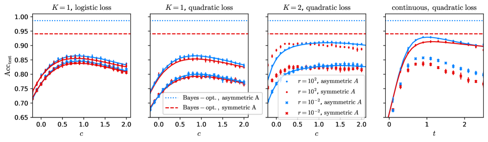
The image presents four separate charts comparing the performance (Acc_test) of different models under varying conditions. Each chart explores a different loss function and parameter setting. The x-axis represents a parameter 'c' in the first three charts and 't' in the last chart. The y-axis, labeled "Acc_test", represents the accuracy score. Two model types are compared: "asymmetric A" and "symmetric A", with different values of 'r' (10^2 and 10^-2). Each chart also includes a "Bayes – opt." baseline, represented by dotted lines, for both asymmetric and symmetric cases.
### Components/Axes
* **Y-axis (all charts):** Acc_test (Accuracy Score), ranging from approximately 0.65 to 1.00.
* **Chart 1:** K = 1, logistic loss; X-axis: c, ranging from 0.0 to 2.0.
* **Chart 2:** K = 1, quadratic loss; X-axis: c, ranging from 0.0 to 2.0.
* **Chart 3:** K = 2, quadratic loss; X-axis: c, ranging from 0.0 to 2.0.
* **Chart 4:** continuous, quadratic loss; X-axis: t, ranging from 0.0 to 2.0.
* **Legend (all charts):**
* `r = 10^2, asymmetric A` (Blue, marked with 'x')
* `r = 10^2, symmetric A` (Red, marked with '+')
* `r = 10^-2, asymmetric A` (Blue, dotted, marked with '.')
* `r = 10^-2, symmetric A` (Red, dotted, marked with '.')
* `Bayes – opt., asymmetric A` (Blue, dashed)
* `Bayes – opt., symmetric A` (Red, dashed)
### Detailed Analysis or Content Details
**Chart 1: K = 1, logistic loss**
* The blue 'x' line (r = 10^2, asymmetric A) starts at approximately 0.72 and increases to around 0.87 at c = 2.0.
* The red '+' line (r = 10^2, symmetric A) starts at approximately 0.70 and increases to around 0.85 at c = 2.0.
* The blue dotted line (r = 10^-2, asymmetric A) starts at approximately 0.73 and increases to around 0.86 at c = 2.0.
* The red dotted line (r = 10^-2, symmetric A) starts at approximately 0.71 and increases to around 0.84 at c = 2.0.
* The blue dashed line (Bayes – opt., asymmetric A) starts at approximately 0.75 and increases to around 0.90 at c = 2.0.
* The red dashed line (Bayes – opt., symmetric A) starts at approximately 0.74 and increases to around 0.89 at c = 2.0.
**Chart 2: K = 1, quadratic loss**
* The blue 'x' line (r = 10^2, asymmetric A) starts at approximately 0.70 and increases rapidly to around 0.92 at c = 1.5, then plateaus at around 0.93 at c = 2.0.
* The red '+' line (r = 10^2, symmetric A) starts at approximately 0.68 and increases rapidly to around 0.90 at c = 1.5, then plateaus at around 0.91 at c = 2.0.
* The blue dotted line (r = 10^-2, asymmetric A) starts at approximately 0.71 and increases to around 0.88 at c = 2.0.
* The red dotted line (r = 10^-2, symmetric A) starts at approximately 0.69 and increases to around 0.87 at c = 2.0.
* The blue dashed line (Bayes – opt., asymmetric A) starts at approximately 0.73 and increases to around 0.94 at c = 2.0.
* The red dashed line (Bayes – opt., symmetric A) starts at approximately 0.72 and increases to around 0.93 at c = 2.0.
**Chart 3: K = 2, quadratic loss**
* The blue 'x' line (r = 10^2, asymmetric A) starts at approximately 0.70 and increases to around 0.94 at c = 2.0.
* The red '+' line (r = 10^2, symmetric A) starts at approximately 0.68 and increases to around 0.92 at c = 2.0.
* The blue dotted line (r = 10^-2, asymmetric A) starts at approximately 0.72 and increases to around 0.88 at c = 2.0.
* The red dotted line (r = 10^-2, symmetric A) starts at approximately 0.70 and increases to around 0.86 at c = 2.0.
* The blue dashed line (Bayes – opt., asymmetric A) starts at approximately 0.74 and increases to around 0.96 at c = 2.0.
* The red dashed line (Bayes – opt., symmetric A) starts at approximately 0.73 and increases to around 0.95 at c = 2.0.
**Chart 4: continuous, quadratic loss**
* The blue 'x' line (r = 10^2, asymmetric A) starts at approximately 0.75 and increases to around 0.98 at t = 1.0, then decreases slightly to around 0.96 at t = 2.0.
* The red '+' line (r = 10^2, symmetric A) starts at approximately 0.73 and increases to around 0.97 at t = 1.0, then decreases slightly to around 0.95 at t = 2.0.
* The blue dotted line (r = 10^-2, asymmetric A) starts at approximately 0.76 and increases to around 0.90 at t = 2.0.
* The red dotted line (r = 10^-2, symmetric A) starts at approximately 0.74 and increases to around 0.88 at t = 2.0.
* The blue dashed line (Bayes – opt., asymmetric A) starts at approximately 0.78 and increases to around 0.99 at t = 1.0, then decreases slightly to around 0.97 at t = 2.0.
* The red dashed line (Bayes – opt., symmetric A) starts at approximately 0.77 and increases to around 0.98 at t = 1.0, then decreases slightly to around 0.96 at t = 2.0.
### Key Observations
* The "Bayes – opt." lines consistently outperform the other models across all charts.
* In the first three charts, the performance of models with r = 10^2 is generally better than those with r = 10^-2.
* The difference between asymmetric and symmetric models is relatively small, especially for the "Bayes – opt." lines.
* Chart 4 shows a peak in performance around t = 1.0 for all models, followed by a slight decrease.
### Interpretation
The charts demonstrate the performance of different models under various loss functions (logistic and quadratic) and parameter settings (K and r). The consistent outperformance of the "Bayes – opt." models suggests they provide a strong baseline for comparison. The choice of 'r' value significantly impacts performance, with larger values (10^2) generally leading to better accuracy, particularly in the first three charts. The slight performance decrease observed in Chart 4 after t = 1.0 could indicate overfitting or a saturation point in the learning process. The relatively small difference between asymmetric and symmetric models suggests that the asymmetry of the model does not have a substantial impact on performance in these scenarios. These results could inform the selection of appropriate model parameters and loss functions for similar tasks.