TECHNICAL ASSET FINGERPRINT
ee07d7ce85fe8c1339d7a345
Click to view fullscreen
Press ESC or click to close
FOUND IN PAPERS
EXPERT: healer-alpha-free VERSION 1
RUNTIME: free/openrouter/healer-alpha
INTEL_VERIFIED
## Multi-Panel Line Chart: Accuracy vs. Regularization Parameter
### Overview
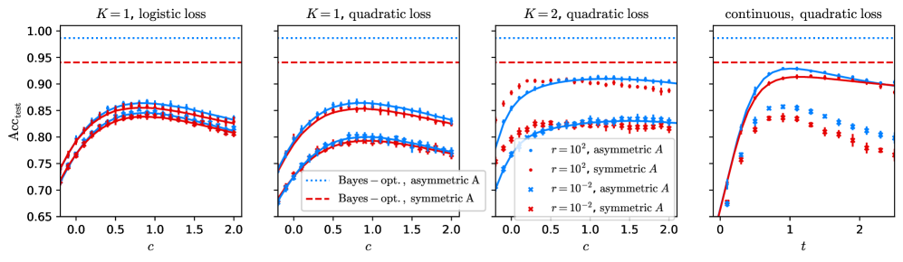
The image displays a set of four line charts arranged horizontally. Each chart plots the test accuracy (`Acc_{cost}`) against a regularization parameter (`c` or `t`) for different machine learning model configurations. The charts compare the effects of loss function type (logistic vs. quadratic), model complexity (`K=1`, `K=2`, continuous), and data distribution symmetry (symmetric vs. asymmetric `A`).
### Components/Axes
* **Overall Structure:** Four subplots in a 1x4 grid.
* **Y-Axis (All Panels):** Labeled `Acc_{cost}`. The scale ranges from 0.65 to 1.00, with major ticks at 0.05 intervals.
* **X-Axis:**
* **Panels 1-3:** Labeled `c`. The scale ranges from 0.0 to 2.0, with major ticks at 0.5 intervals.
* **Panel 4:** Labeled `t`. The scale ranges from 0 to 2, with major ticks at 1 intervals.
* **Legend (Located in Panel 2, bottom-right):**
* **Blue dotted line:** `Bayes - opt., asymmetric A`
* **Red dashed line:** `Bayes - opt., symmetric A`
* **Blue circle marker:** `r = 10^2, asymmetric A`
* **Red circle marker:** `r = 10^2, symmetric A`
* **Blue 'x' marker:** `r = 10^{-2}, asymmetric A`
* **Red 'x' marker:** `r = 10^{-2}, symmetric A`
* **Panel Titles:**
* **Panel 1 (Left):** `K = 1, logistic loss`
* **Panel 2:** `K = 1, quadratic loss`
* **Panel 3:** `K = 2, quadratic loss`
* **Panel 4 (Right):** `continuous, quadratic loss`
### Detailed Analysis
**Panel 1: K = 1, logistic loss**
* **Trend:** All four data series (blue/red circles and 'x's) follow a similar inverted-U shape. Accuracy increases from `c=0.0` to a peak around `c=0.8-1.0`, then gradually decreases.
* **Data Points (Approximate):**
* At `c=0.0`, all series start near `Acc ≈ 0.71`.
* Peak accuracy for all series is between `0.84` and `0.86`.
* At `c=2.0`, accuracy for all series falls to between `0.80` and `0.83`.
* **Bayes-Optimal Lines:** The blue dotted line (`asymmetric A`) is constant at `Acc ≈ 0.99`. The red dashed line (`symmetric A`) is constant at `Acc ≈ 0.94`.
**Panel 2: K = 1, quadratic loss**
* **Trend:** Similar inverted-U shape as Panel 1, but the curves are lower and the peak is less pronounced. The separation between the `r=10^2` (circles) and `r=10^{-2}` ('x's) series is more distinct.
* **Data Points (Approximate):**
* At `c=0.0`, series start between `Acc ≈ 0.68` and `0.72`.
* The `r=10^2` series (circles) peak around `c=0.8` with `Acc ≈ 0.86`.
* The `r=10^{-2}` series ('x's) peak around `c=0.8` with `Acc ≈ 0.80`.
* At `c=2.0`, the `r=10^2` series are near `Acc ≈ 0.83`, and the `r=10^{-2}` series are near `Acc ≈ 0.77`.
* **Bayes-Optimal Lines:** Identical to Panel 1 (Blue dotted `≈0.99`, Red dashed `≈0.94`).
**Panel 3: K = 2, quadratic loss**
* **Trend:** The curves rise more steeply from `c=0.0` and plateau earlier (around `c=0.5-1.0`) compared to K=1 models. The `r=10^2` series (circles) achieve significantly higher accuracy than the `r=10^{-2}` series ('x's).
* **Data Points (Approximate):**
* At `c=0.0`, series start between `Acc ≈ 0.70` and `0.75`.
* The `r=10^2` series (circles) plateau between `Acc ≈ 0.90` and `0.92`.
* The `r=10^{-2}` series ('x's) plateau between `Acc ≈ 0.82` and `0.84`.
* Accuracy remains relatively stable from `c=1.0` to `c=2.0`.
* **Bayes-Optimal Lines:** Identical to previous panels.
**Panel 4: continuous, quadratic loss**
* **Trend:** This panel shows a different dynamic. The `r=10^2` series (circles) rise sharply to a peak near `t=1.0` and then decline. The `r=10^{-2}` series ('x's) rise to a lower peak and decline more sharply.
* **Data Points (Approximate):**
* At `t=0`, all series start near `Acc ≈ 0.65`.
* The `r=10^2` series (circles) peak near `t=1.0` with `Acc ≈ 0.92`.
* The `r=10^{-2}` series ('x's) peak near `t=0.8` with `Acc ≈ 0.85`.
* At `t=2.0`, the `r=10^2` series are near `Acc ≈ 0.90`, and the `r=10^{-2}` series are near `Acc ≈ 0.78`.
* **Bayes-Optimal Lines:** Identical to previous panels.
### Key Observations
1. **Consistent Bayes-Optimal Benchmark:** The theoretical maximum accuracy (Bayes-optimal) is consistently higher for the asymmetric data distribution (`A`) than for the symmetric one across all model types.
2. **Impact of Regularization (`c`):** For finite `K` models (Panels 1-3), there is an optimal intermediate value of the regularization parameter `c` that maximizes test accuracy. Too little or too much regularization hurts performance.
3. **Effect of Model Complexity (`K`):** Moving from `K=1` (Panels 1 & 2) to `K=2` (Panel 3) allows models to achieve higher accuracy, closer to the Bayes-optimal limit, especially for the `r=10^2` setting.
4. **Parameter `r` Sensitivity:** The parameter `r` (likely a noise or scale parameter) has a major impact. Models with `r=10^2` (circles) consistently outperform those with `r=10^{-2}` ('x's) across all configurations.
5. **Loss Function Comparison:** For `K=1`, the logistic loss (Panel 1) yields slightly higher peak accuracy (`≈0.86`) than the quadratic loss (Panel 2, `≈0.86` for `r=10^2`), but the quadratic loss curves show more separation between the `r` values.
6. **Continuous Model Behavior:** The continuous model (Panel 4) shows a distinct peak-and-decline pattern with respect to `t`, suggesting a different optimal operating point compared to the finite `K` models parameterized by `c`.
### Interpretation
This set of charts investigates the generalization performance of models with varying complexity (`K=1`, `K=2`, continuous) under different loss functions and data distributions. The key takeaway is the interplay between **model complexity**, **regularization strength** (`c` or `t`), and a **data/noise parameter** (`r`).
* **The Bias-Variance Tradeoff:** The inverted-U curves in Panels 1-3 are a classic visualization of the bias-variance tradeoff. As regularization (`c`) increases, model variance decreases but bias may increase. The peak represents the optimal balance for test set generalization.
* **Model Capacity Matters:** More complex models (`K=2`, continuous) can achieve higher accuracy, approaching the Bayes-optimal bound more closely than simpler models (`K=1`). However, they also require careful tuning of the regularization parameter.
* **Data Distribution Impact:** The consistently higher Bayes-optimal line for asymmetric `A` suggests that the underlying classification task is inherently easier when the data distribution is asymmetric. All models reflect this, performing better on the asymmetric task (blue markers/lines) than the symmetric one (red markers/lines) for the same `r` value.
* **The Role of `r`:** The parameter `r` appears to be a critical factor controlling the difficulty of the learning problem or the model's sensitivity. A higher `r` (`10^2`) leads to substantially better and more robust performance across all model types compared to a low `r` (`10^{-2}`). This could correspond to a signal-to-noise ratio or a scaling factor in the data generation process.
In summary, the figure demonstrates that achieving near-optimal performance requires selecting a model with sufficient complexity, tuning regularization appropriately, and is fundamentally constrained by the properties of the data distribution (`A` and `r`). The continuous model exhibits a different sensitivity profile to its complexity parameter `t`.
DECODING INTELLIGENCE...