## Histogram: Distribution of Thinking Token Usage
### Overview
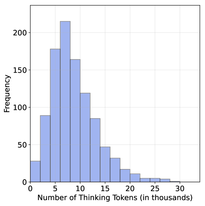
The image displays a histogram illustrating the frequency distribution of "Thinking Tokens" used, measured in thousands. The chart shows a right-skewed distribution, indicating that most instances involve a moderate number of thinking tokens, with a long tail extending toward higher token counts.
### Components/Axes
* **Chart Type:** Histogram (vertical bars).
* **X-Axis (Horizontal):**
* **Label:** "Number of Thinking Tokens (in thousands)"
* **Scale:** Linear scale from 0 to 30, with major tick marks and labels at intervals of 5 (0, 5, 10, 15, 20, 25, 30).
* **Bin Width:** Each bar represents a range of 2.5 thousand tokens (e.g., 0-2.5, 2.5-5, 5-7.5, etc.).
* **Y-Axis (Vertical):**
* **Label:** "Frequency"
* **Scale:** Linear scale from 0 to over 200, with major tick marks and labels at intervals of 50 (0, 50, 100, 150, 200).
* **Legend:** None present. The chart represents a single data series.
* **Visual Style:** Bars are filled with a light blue color and have a thin, dark outline. The background is white with a light gray grid aligned with the major y-axis ticks.
### Detailed Analysis
The following table reconstructs the approximate frequency for each token range (bin), derived from visual inspection of the bar heights against the y-axis scale. Values are approximate.
| Thinking Tokens (in thousands) | Approximate Frequency |
| :--- | :--- |
| 0 - 2.5 | 30 |
| 2.5 - 5 | 90 |
| 5 - 7.5 | 180 |
| **7.5 - 10** | **~215** (Peak) |
| 10 - 12.5 | 165 |
| 12.5 - 15 | 120 |
| 15 - 17.5 | 85 |
| 17.5 - 20 | 45 |
| 20 - 22.5 | 30 |
| 22.5 - 25 | 15 |
| 25 - 27.5 | 10 |
| 27.5 - 30 | 5 |
**Trend Verification:** The visual trend is a rapid rise to a peak, followed by a steady decline. The frequency increases sharply from the 0-2.5k bin to the 7.5-10k bin (the mode), then decreases progressively for each subsequent higher token range, forming a long right tail.
### Key Observations
1. **Modal Peak:** The most common usage range is between 7,500 and 10,000 thinking tokens.
2. **Right Skew:** The distribution is positively skewed. The tail on the right side (higher token counts) is longer and more gradual than the left side.
3. **Concentration:** The vast majority of instances (the bulk of the distribution) fall between 2,500 and 17,500 tokens.
4. **Rare High Usage:** Instances requiring more than 20,000 tokens are relatively infrequent, and those exceeding 25,000 are very rare.
5. **Lower Bound:** There is a non-zero frequency for the lowest bin (0-2.5k), indicating some processes complete with minimal thinking tokens.
### Interpretation
This histogram provides a quantitative profile of computational "effort" or complexity, as measured by thinking token consumption.
* **Typical Process Complexity:** The concentration of data between 5k and 15k tokens suggests that the standard or most common tasks processed by this system require a moderate amount of sequential reasoning or computation.
* **Efficiency and Outliers:** The sharp peak indicates a well-defined typical operating range. The long right tail is significant; it demonstrates that while rare, there exists a subset of tasks that are substantially more complex, requiring 2-3 times the token usage of a typical task. This could represent edge cases, highly intricate problems, or potential inefficiencies in certain processes.
* **System Design Implication:** The distribution informs resource allocation. System capacity should be designed to comfortably handle the 7.5k-10k token range for peak load, while also having the capability (e.g., timeout limits, memory allocation) to accommodate the less frequent but much more demanding tasks in the 20k+ range without failure.
* **Absence of a Lower Mode:** The lack of a significant peak near zero suggests that very few tasks are trivial; most require some substantive "thinking."