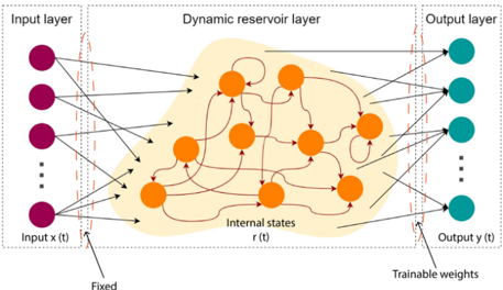
## Diagram: Reservoir Computing Network ### Overview The image is a diagram illustrating the architecture of a reservoir computing network. It consists of three main layers: an input layer, a dynamic reservoir layer, and an output layer. The diagram shows the connections between these layers and highlights the fixed and trainable weights within the network. ### Components/Axes * **Input Layer:** Located on the left side of the diagram. Contains a series of purple nodes. Labeled "Input layer" at the top and "Input x(t)" at the bottom. * **Dynamic Reservoir Layer:** Located in the center of the diagram. Contains a network of interconnected orange nodes within a shaded orange region. Labeled "Dynamic reservoir layer" at the top and "Internal states r(t)" at the bottom. * **Output Layer:** Located on the right side of the diagram. Contains a series of teal nodes. Labeled "Output layer" at the top and "Output y(t)" at the bottom. * **Connections:** Arrows indicate the flow of information between the layers. Connections from the input layer to the reservoir layer and from the reservoir layer to the output layer. The reservoir layer also contains internal connections. * **Weights:** The connections between the input layer and the reservoir layer are labeled as "Fixed". The connections between the reservoir layer and the output layer are labeled as "Trainable weights". ### Detailed Analysis * **Input Layer:** The input layer consists of at least 3 purple nodes, with an ellipsis indicating that there may be more. Each node in the input layer has connections to multiple nodes in the dynamic reservoir layer. * **Dynamic Reservoir Layer:** The dynamic reservoir layer is the core of the network. It consists of approximately 10 orange nodes interconnected in a complex, recurrent manner. The connections within the reservoir are represented by curved arrows, indicating feedback loops. The entire reservoir is contained within a shaded orange region. * **Output Layer:** The output layer consists of at least 3 teal nodes, with an ellipsis indicating that there may be more. Each node in the output layer receives input from multiple nodes in the dynamic reservoir layer. * **Connections:** The connections between the input layer and the reservoir layer appear to be randomly distributed. The connections between the reservoir layer and the output layer are also distributed. * **Weights:** The diagram explicitly labels the weights between the input and reservoir layers as "Fixed," implying that these connections are not adjusted during training. The weights between the reservoir and output layers are labeled as "Trainable weights," indicating that these connections are adjusted during the training process. ### Key Observations * The dynamic reservoir layer is a complex, recurrent network. * The connections between the input layer and the reservoir layer are fixed. * The connections between the reservoir layer and the output layer are trainable. ### Interpretation The diagram illustrates the fundamental architecture of a reservoir computing network. The key idea behind reservoir computing is to use a fixed, randomly connected recurrent neural network (the dynamic reservoir layer) to map the input signal into a higher-dimensional space. The output layer is then trained to read out the desired output from this high-dimensional representation. The fixed weights between the input and reservoir layers allow the reservoir to act as a non-linear feature extractor. The trainable weights between the reservoir and output layers allow the network to learn the mapping from the reservoir's internal states to the desired output. The recurrent connections within the reservoir allow the network to process temporal data, making it suitable for tasks such as speech recognition, time series prediction, and control. The complexity of the reservoir's internal connections is crucial for its ability to capture the dynamics of the input signal.