## Diagram: Reservoir Computing Architecture
### Overview
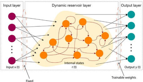
The diagram illustrates a reservoir computing architecture, a type of recurrent neural network (RNN) structure. It consists of three primary components: an input layer, a dynamic reservoir layer, and an output layer. Arrows indicate directional flow and connections between components, with annotations specifying fixed vs. trainable parameters.
### Components/Axes
1. **Input Layer**:
- **Nodes**: Purple circles labeled "Input x(t)" (time-dependent input).
- **Connections**: Black arrows with red dashed outlines connecting inputs to the reservoir.
- **Annotations**: "Fixed" (weights between input and reservoir are static).
2. **Dynamic Reservoir Layer**:
- **Nodes**: Orange circles labeled "Internal states r(t)".
- **Connections**: Red arrows forming a dense, recurrent network (self-connections and inter-node connections).
- **Annotations**: "Internal states" (dynamic, time-dependent processing).
3. **Output Layer**:
- **Nodes**: Teal circles labeled "Output y(t)".
- **Connections**: Black arrows with red dashed outlines from the reservoir to outputs.
- **Annotations**: "Trainable weights" (weights between reservoir and output are optimized during training).
4. **Legend/Annotations**:
- **Color Coding**:
- Purple: Input layer.
- Orange: Reservoir nodes.
- Teal: Output layer.
- Red: Reservoir internal connections.
- Black: Input/output layer connections.
- **Key Labels**:
- "Fixed" (input-reservoir weights).
- "Trainable weights" (reservoir-output weights).
### Detailed Analysis
- **Input Layer**:
- Receives time-series data `x(t)`.
- Fixed weights ensure the input pattern is preserved without modification during training.
- **Reservoir Layer**:
- Processes inputs through chaotic, high-dimensional dynamics (`r(t)`).
- Dense recurrent connections (red arrows) enable complex temporal pattern learning.
- No explicit bias terms or activation functions labeled.
- **Output Layer**:
- Maps reservoir states to desired outputs `y(t)`.
- Trainable weights allow the network to learn task-specific mappings from the reservoir's dynamics.
### Key Observations
1. **Fixed vs. Trainable Weights**:
- Input-reservoir connections are static ("Fixed").
- Reservoir-output connections are optimized ("Trainable weights").
2. **Reservoir Dynamics**:
- The chaotic, high-connectivity structure suggests a "black box" for feature extraction.
- No explicit time-delay elements or gating mechanisms (e.g., LSTM/GRU) are shown.
3. **Output Structure**:
- Output nodes are directly connected to reservoir states, implying linear readout (common in reservoir computing).
### Interpretation
This architecture demonstrates the core principles of reservoir computing:
- **Fixed Input Weights**: Preserve input patterns while allowing the reservoir to learn temporal dynamics.
- **Trainable Output Weights**: Enable task-specific learning by adjusting the readout layer.
- **Reservoir Complexity**: The dense, recurrent connections create a high-dimensional, chaotic space for feature representation.
The diagram emphasizes the separation of timescale learning (reservoir dynamics) and parameter optimization (output weights), a hallmark of reservoir computing's efficiency in handling sequential data. The absence of explicit activation functions or regularization terms suggests a focus on the theoretical framework rather than implementation details.