\n
## 3D Surface Plot: Free Energy Landscape
### Overview
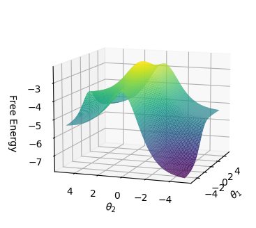
The image depicts a 3D surface plot representing a free energy landscape. The plot visualizes the relationship between two angular parameters, θ₁ and θ₂, and the corresponding free energy. The surface is colored to indicate the free energy value, with warmer colors (yellow/green) representing lower free energy and cooler colors (blue/purple) representing higher free energy.
### Components/Axes
* **X-axis:** θ₁ (Theta 1), ranging approximately from -4 to 4.
* **Y-axis:** θ₂ (Theta 2), ranging approximately from -4 to 4.
* **Z-axis:** Free Energy, ranging approximately from -7 to -3.
* **Color Scale:** Represents Free Energy, with a gradient from purple (high energy) to yellow/green (low energy).
### Detailed Analysis
The surface exhibits a complex topography with multiple local minima and maxima.
* **Main Minimum:** A prominent minimum is located near θ₁ ≈ 0 and θ₂ ≈ 0, with a free energy value of approximately -3. This is indicated by the yellow/green color in that region.
* **Secondary Minima:** There are two secondary minima located approximately at:
* θ₁ ≈ 3, θ₂ ≈ 2, with a free energy of approximately -4.
* θ₁ ≈ -3, θ₂ ≈ -2, with a free energy of approximately -4.
* **Saddle Points:** Several saddle points are visible, connecting the minima. These are indicated by regions where the color changes rapidly.
* **Maximum:** A maximum is located approximately at θ₁ ≈ -4 and θ₂ ≈ 4, with a free energy of approximately -7.
* **Trend:** The surface generally slopes downward from the upper-right to the lower-left, indicating a decreasing free energy in that direction.
### Key Observations
* The landscape is not smooth; it has several distinct features.
* The primary minimum suggests a stable state at θ₁ ≈ 0 and θ₂ ≈ 0.
* The secondary minima suggest metastable states.
* The presence of saddle points indicates pathways between different states.
### Interpretation
This plot likely represents the free energy landscape of a system with two degrees of freedom, represented by the angles θ₁ and θ₂. The minima on the landscape correspond to stable or metastable states of the system. The height of the energy barriers (represented by the saddle points) determines the rate of transitions between these states. The system will tend to reside in the minimum energy state, but thermal fluctuations can allow it to overcome the energy barriers and explore other states. The shape of the landscape provides insights into the dynamics and stability of the system. The plot suggests that the system has a preferred configuration around θ₁ ≈ 0 and θ₂ ≈ 0, but can also exist in other configurations with slightly higher energy. The complexity of the landscape indicates that the system's behavior may be non-trivial.