## 3D Surface Plot: Free Energy Landscape as a Function of θ₁ and θ₂
### Overview
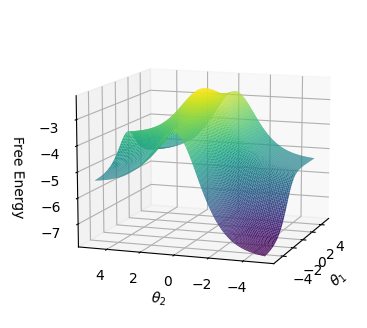
The image depicts a 3D surface plot representing a free energy landscape with two variables, θ₁ (horizontal axis) and θ₂ (depth axis). The vertical axis represents free energy values ranging from -7 to -3. The surface exhibits a complex topography with multiple peaks, valleys, and saddle points, colored in a gradient from purple (lowest energy) to yellow (highest energy).
### Components/Axes
- **Axes Labels**:
- **X-axis (θ₁)**: Ranges from -4 to 4 in increments of 2.
- **Y-axis (θ₂)**: Ranges from -4 to 4 in increments of 2.
- **Z-axis (Free Energy)**: Ranges from -7 to -3 in increments of 1.
- **Color Gradient**:
- Purple → Yellow: Represents increasing free energy values (no explicit legend, but inferred from color mapping).
- **Grid Lines**: Black grid lines define the 3D coordinate system.
### Detailed Analysis
1. **Highest Energy Point**:
- **Location**: θ₁ ≈ 0, θ₂ ≈ 0.
- **Free Energy**: Approximately -3 (uncertainty: ±0.5).
- **Color**: Yellow (consistent with highest energy).
2. **Lowest Energy Point**:
- **Location**: θ₁ ≈ -4, θ₂ ≈ -4.
- **Free Energy**: Approximately -7 (uncertainty: ±0.5).
- **Color**: Purple (consistent with lowest energy).
3. **Saddle Point**:
- **Location**: θ₁ ≈ 2, θ₂ ≈ 2.
- **Free Energy**: Approximately -4.5 (uncertainty: ±0.5).
- **Color**: Green (intermediate energy).
4. **Additional Features**:
- **Peaks**:
- θ₁ ≈ -2, θ₂ ≈ 2: Free energy ≈ -5 (green).
- θ₁ ≈ 2, θ₂ ≈ -2: Free energy ≈ -5 (green).
- **Valleys**:
- θ₁ ≈ -3, θ₂ ≈ 3: Free energy ≈ -6 (dark blue).
- θ₁ ≈ 3, θ₂ ≈ -3: Free energy ≈ -6 (dark blue).
### Key Observations
- The system exhibits **multiple metastable states** (valleys) and **transition states** (saddle points).
- The energy landscape is **asymmetric**, with the global minimum at θ₁ = -4, θ₂ = -4 and the local minimum at θ₁ = 0, θ₂ = 0.
- The saddle point at θ₁ = 2, θ₂ = 2 acts as a **barrier** between the global and local minima.
### Interpretation
This free energy landscape suggests a system with **competing stable and unstable states**. The global minimum at θ₁ = -4, θ₂ = -4 represents the most thermodynamically favorable configuration, while the local minimum at θ₁ = 0, θ₂ = 0 indicates a metastable state. The saddle point at θ₁ = 2, θ₂ = 2 implies a **transition barrier** that must be overcome for the system to shift between these states. The asymmetry in the landscape highlights **directional energy gradients**, which could drive the system toward specific configurations under external perturbations (e.g., temperature changes or external fields). The absence of a uniform energy distribution suggests **nonlinear interactions** between θ₁ and θ₂, potentially indicative of complex molecular or physical systems (e.g., protein folding, chemical reactions, or phase transitions).