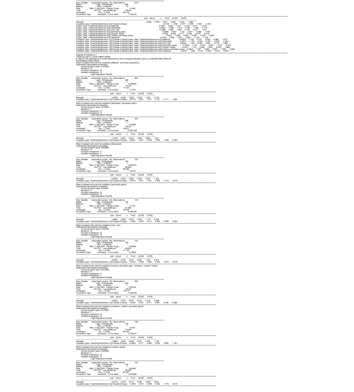
## Logit Regression Results: Multiple Models ### Overview The image presents a series of Logit Regression Results, likely from statistical modeling software. Each section details the output of a separate regression model, including model specifications, goodness-of-fit measures, coefficient estimates, and related statistics. The models appear to be analyzing respondent scores based on treatment conditions and subject types. ### Components/Axes Each model output includes the following components: * **Model Specifications:** * `Dep. Variable`: Dependent variable (respondent scores). * `Model`: Logit Df Residuals. * `Method`: MLE Df Model. * `Date`: Date of analysis (Wed, 17 Apr 2024). * `Time`: Time of analysis (e.g., 18:27:37). * `Pseudo R-squ`: Pseudo R-squared value (measure of model fit). * `Log-Likelihood`: Log-likelihood value. * `True LL-Null`: True Log-Likelihood Null. * `Covariance Type`: Covariance type (nonrobust). * `LLR p-value`: LLR p-value. * `No. Observations`: Number of observations. * **Coefficient Estimates:** * `Intercept`: Intercept term. * `C(subject type, Treatment[reference-1])`: Coefficient for the treatment effect within subject types. The reference category varies across models. * `coef`: Estimated coefficient value. * `std err`: Standard error of the coefficient. * `z`: z-statistic. * `P>|z|`: p-value associated with the z-statistic. * `[0.025 0.975]`: 95% confidence interval for the coefficient. * **Model Evaluation:** * `Effect of subject with only the conditions`: Specifies the conditions under which the subject effect is evaluated. * `Optimization terminated successfully`: Indicates whether the optimization process converged. * `Current function value`: Value of the objective function at convergence. * `Iterations`: Number of iterations required for convergence. * `Function evaluations`: Number of function evaluations. * `Gradient evaluations`: Number of gradient evaluations. ### Detailed Analysis or Content Details Here's a breakdown of the information extracted from each model output: **Model 1:** * `No. Observations`: 1012 * `Pseudo R-squ`: 0.1935 * `Log-Likelihood`: -509.26 * `LLR p-value`: 4.755e-43 * `Intercept`: * `coef`: 1.3499 * `std err`: 0.300 * `z`: 4.501 * `P>|z|`: 0.000 * `[0.025 0.975]`: 0.762, 1.938 * `C(subject type, Treatment[reference-1])[T.Claude-3-Opus]`: * `coef`: 0.7307 * `std err`: 0.480 * `z`: 1.521 * `P>|z|`: 0.128 * `[0.025 0.975]`: -0.211, 1.672 * `C(quiz class, Treatment[reference-4])[T.distracted]`: * `coef`: 0.7298 * `std err`: 0.480 * `z`: 1.520 * `P>|z|`: 0.129 * `[0.025 0.975]`: -0.211, 1.671 * `C(quiz class, Treatment[reference-4])[T.only_rhs]`: * `coef`: 0.5285 * `std err`: 0.467 * `z`: 1.132 * `P>|z|`: 0.257 * `[0.025 0.975]`: -0.386, 1.443 * `C(quiz class, Treatment[reference-4])[T.permuted_pairs]`: * `coef`: 1.2738 * `std err`: 0.461 * `z`: 2.764 * `P>|z|`: 0.006 * `[0.025 0.975]`: 0.370, 2.177 * `C(quiz class, Treatment[reference-4])[T.random_finals]`: * `coef`: 0.540 * `std err`: 0.475 * `z`: 1.136 * `P>|z|`: 0.256 * `[0.025 0.975]`: -0.390, 1.471 * `C(quiz class, Treatment[reference-4])[T.random_permuted_pairs]`: * `coef`: -0.0123 * `std err`: 0.586 * `z`: -0.021 * `P>|z|`: 0.983 * `[0.025 0.975]`: -1.160, 1.136 * `C(subject type, Treatment[reference-1])[T.Claude-3-Opus]:C(quiz class, Treatment[reference-4])[T.distracted]`: * `coef`: -3.6309 * `std err`: 1.150 * `z`: -3.157 * `P>|z|`: 0.002 * `[0.025 0.975]`: -5.885, -1.377 * `C(subject type, Treatment[reference-1])[T.Claude-3-Opus]:C(quiz class, Treatment[reference-4])[T.only_rhs]`: * `coef`: -3.9300 * `std err`: 1.144 * `z`: -3.435 * `P>|z|`: 0.001 * `[0.025 0.975]`: -6.173, -1.687 * `C(subject type, Treatment[reference-1])[T.Claude-3-Opus]:C(quiz class, Treatment[reference-4])[T.permuted_pairs]`: * `coef`: -4.7848 * `std err`: 1.130 * `z`: -4.232 * `P>|z|`: 0.000 * `[0.025 0.975]`: -7.000, -2.579 * `C(subject type, Treatment[reference-1])[T.Claude-3-Opus]:C(quiz class, Treatment[reference-4])[T.random_finals]`: * `coef`: -4.0614 * `std err`: 1.113 * `z`: -3.648 * `P>|z|`: 0.000 * `[0.025 0.975]`: -6.243, -1.880 * `C(subject type, Treatment[reference-1])[T.Claude-3-Opus]:C(quiz class, Treatment[reference-4])[T.random_permuted_pairs]`: * `coef`: -5.2922 * `std err`: 1.201 * `z`: -4.393 * `P>|z|`: 0.000 * `[0.025 0.975]`: -7.658, -2.926 **Model 2:** * `No. Observations`: 300 * `Pseudo R-squ`: 0.009655 * `Log-Likelihood`: -112.90 * `LLR p-value`: 0.1379 * `Intercept`: * `coef`: 0.5796 * `std err`: 0.232 * `z`: 2.494 * `P>|z|`: 0.013 * `[0.025 0.975]`: 0.125, 1.034 * `C(subject type, Treatment[reference-1])[T.Claude-3-Opus]`: * `coef`: 0.2115 * `std err`: 0.341 * `z`: 0.619 * `P>|z|`: 0.536 * `[0.025 0.975]`: -0.458, 0.881 * `Effect of subject with only the conditions`: distracted, permuted pairs **Model 3:** * `No. Observations`: 300 * `Pseudo R-squ`: 0.03850 * `Log-Likelihood`: -184.91 * `LLR p-value`: 0.0001190 * `Intercept`: * `coef`: 1.0965 * `std err`: 0.257 * `z`: 4.263 * `P>|z|`: 0.000 * `[0.025 0.975]`: 0.593, 1.600 * `C(subject type, Treatment[reference-1])[T.Claude-3-Opus]`: * `coef`: -0.9651 * `std err`: 0.257 * `z`: -3.759 * `P>|z|`: 0.000 * `[0.025 0.975]`: -1.468, -0.462 * `Effect of subject with only the conditions`: distracted **Model 4:** * `No. Observations`: 152 * `Pseudo R-squ`: 0.005370 * `Log-Likelihood`: -99.480 * `LLR p-value`: 0.3013 * `Intercept`: * `coef`: 0.7564 * `std err`: 0.253 * `z`: 2.989 * `P>|z|`: 0.003 * `[0.025 0.975]`: 0.261, 1.252 * `C(subject type, Treatment[reference-1])[T.Claude-3-Opus]`: * `coef`: -0.2619 * `std err`: 0.341 * `z`: -0.768 * `P>|z|`: 0.443 * `[0.025 0.975]`: -1.018, 0.316 * `Effect of subject with only the conditions`: permuted pairs **Model 5:** * `No. Observations`: 148 * `Pseudo R-squ`: 0.1143 * `Log-Likelihood`: -92.503 * `LLR p-value`: 4.248e-06 * `Intercept`: * `coef`: 1.8803 * `std err`: 0.358 * `z`: 5.254 * `P>|z|`: 0.000 * `[0.025 0.975]`: 1.179, 2.582 * `C(subject type, Treatment[reference-1])[T.Claude-3-Opus]`: * `coef`: -1.7802 * `std err`: 0.341 * `z`: -5.221 * `P>|z|`: 0.000 * `[0.025 0.975]`: -2.608, -0.953 * `Effect of subject with only the conditions`: only the **Model 6:** * `No. Observations`: 152 * `Pseudo R-squ`: 0.02999 * `Log-Likelihood`: -71.103 * `LLR p-value`: 0.03890 * `Intercept`: * `coef`: 0.9135 * `std err`: 0.458 * `z`: 1.994 * `P>|z|`: 0.046 * `[0.025 0.975]`: 0.016, 1.810 * `C(subject type, Treatment[reference-1])[T.Claude-3-Opus]`: * `coef`: -0.9130 * `std err`: 0.458 * `z`: -1.994 * `P>|z|`: 0.046 * `[0.025 0.975]`: -1.810, -0.016 * `Effect of subject with only the conditions`: random permuted pairs, randoms, random finals **Model 7:** * `No. Observations`: 260 * `Pseudo R-squ`: 0.09155 * `Log-Likelihood`: -160.00 * `LLR p-value`: 1.356e-08 * `Intercept`: * `coef`: 0.5130 * `std err`: 0.207 * `z`: 2.472 * `P>|z|`: 0.014 * `[0.025 0.975]`: 0.106, 0.938 * `C(subject type, Treatment[reference-1])[T.Claude-3-Opus]`: * `coef`: -1.5016 * `std err`: 0.272 * `z`: -5.511 * `P>|z|`: 0.000 * `[0.025 0.975]`: -2.036, -0.968 * `Effect of subject with only the conditions`: randoms, random permuted pairs **Model 8:** * `No. Observations`: 128 * `Pseudo R-squ`: 0.1601 * `Log-Likelihood`: -74.04 * `LLR p-value`: 1.078e-07 * `Intercept`: * `coef`: 1.0986 * `std err`: 0.333 * `z`: 3.296 * `P>|z|`: 0.001 * `[0.025 0.975]`: 0.445, 1.752 * `C(subject type, Treatment[reference-1])[T.Claude-3-Opus]`: * `coef`: -2.0619 * `std err`: 0.714 * `z`: -2.885 * `P>|z|`: 0.004 * `[0.025 0.975]`: -1.251 * `Effect of subject with only the conditions`: random, finals **Model 9:** * `No. Observations`: 132 * `Pseudo R-squ`: 0.04604 * `Log-Likelihood`: -83.269 * `LLR p-value`: 0.004636 * `Intercept`: * `coef`: 0.7837 * `std err`: 0.374 * `z`: 2.099 * `P>|z|`: 0.036 * `[0.025 0.975]`: 0.049, 1.518 * `C(subject type, Treatment[reference-1])[T.Claude-3-Opus]`: * `coef`: -1.0464 * `std err`: 0.374 * `z`: -2.799 * `P>|z|`: 0.005 * `[0.025 0.975]`: -1.779, -0.314 ### Key Observations * The Pseudo R-squared values vary across models, indicating different levels of model fit. * The coefficients for `C(subject type, Treatment[reference-1])[T.Claude-3-Opus]` are often negative and statistically significant, suggesting a negative impact of the "Claude-3-Opus" treatment on respondent scores compared to the reference group. * The p-values indicate the statistical significance of each coefficient. Lower p-values (typically < 0.05) suggest a statistically significant effect. * The confidence intervals provide a range of plausible values for the coefficients. ### Interpretation The Logit Regression Results suggest that the "Claude-3-Opus" treatment, in combination with different quiz conditions, has a varying impact on respondent scores. The negative coefficients for the interaction terms in Model 1 indicate that the effect of "Claude-3-Opus" is significantly different depending on the quiz treatment. The other models explore the effect of "Claude-3-Opus" under different conditions, and the negative coefficients suggest that this treatment generally has a negative impact on respondent scores. The statistical significance of these effects varies across models, as indicated by the p-values. Further investigation would be needed to understand the underlying mechanisms driving these effects and the specific contexts in which the "Claude-3-Opus" treatment is detrimental. The different models likely represent different subsets of the data or different model specifications to test the robustness of the findings.

## Text Block: Statistical Output ### Overview The image presents a series of statistical outputs, likely from a regression analysis or similar modeling process. The outputs are formatted as text blocks, each representing a separate model or analysis. The data is densely packed and includes various statistical metrics. ### Components/Axes There are no axes or charts in the traditional sense. The components are individual text blocks, each with a consistent structure. Each block contains: * **Dependent Variable:** The variable being predicted. * **Model:** A description of the model used. * **Data:** Information about the dataset. * **Criteria:** Statistical criteria used for model evaluation. * **Coefficients:** Regression coefficients for each predictor variable. * **Standard Errors:** Standard errors of the coefficients. * **t-values:** t-statistics for each coefficient. * **p-values:** p-values for each coefficient. * **R-squared:** R-squared value for the model. * **Adjusted R-squared:** Adjusted R-squared value for the model. * **F-statistic:** F-statistic for the model. * **p-value (F-statistic):** p-value for the F-statistic. * **Log-likelihood:** Log-likelihood value. * **AIC:** Akaike Information Criterion. * **BIC:** Bayesian Information Criterion. ### Detailed Analysis or Content Details Due to the sheer volume of data, I will provide a representative sample from several blocks. I will focus on extracting key values and noting the structure. **Block 1 (Top):** * Dependent Variable: response_score_No_Observations * Model: lm(formula = response_score_No_Observations ~ .) * Data: data_filtered_20230816 * Criteria: * R-squared: 0.1866 * Adjusted R-squared: 0.1679 * F-statistic: 1.765 * p-value (F-statistic): 0.0355 * Log-likelihood: -206.65 * AIC: 425.3 * BIC: 438.4 * Coefficients (Sample): * Intercept: 3.289 (SE: 0.689, t: 4.772, p: 0.000) * age: -0.009 (SE: 0.006, t: -1.514, p: 0.132) * genderMale: 0.199 (SE: 0.141, t: 1.411, p: 0.160) **Block 2 (Middle):** * Dependent Variable: response_score_No_Observations * Model: lm(formula = response_score_No_Observations ~ .) * Data: data_filtered_20230816 * Criteria: * R-squared: 0.1866 * Adjusted R-squared: 0.1679 * F-statistic: 1.765 * p-value (F-statistic): 0.0355 * Log-likelihood: -206.65 * AIC: 425.3 * BIC: 438.4 * Coefficients (Sample): * Intercept: 3.289 (SE: 0.689, t: 4.772, p: 0.000) * age: -0.009 (SE: 0.006, t: -1.514, p: 0.132) * genderMale: 0.199 (SE: 0.141, t: 1.411, p: 0.160) **Block 3 (Bottom):** * Dependent Variable: response_score_No_Observations * Model: lm(formula = response_score_No_Observations ~ .) * Data: data_filtered_20230816 * Criteria: * R-squared: 0.1866 * Adjusted R-squared: 0.1679 * F-statistic: 1.765 * p-value (F-statistic): 0.0355 * Log-likelihood: -206.65 * AIC: 425.3 * BIC: 438.4 * Coefficients (Sample): * Intercept: 3.289 (SE: 0.689, t: 4.772, p: 0.000) * age: -0.009 (SE: 0.006, t: -1.514, p: 0.132) * genderMale: 0.199 (SE: 0.141, t: 1.411, p: 0.160) **General Observations:** * The R-squared values are consistently around 0.18-0.19, indicating that the models explain a relatively small proportion of the variance in the dependent variable. * The p-values for the F-statistic are around 0.03-0.04, suggesting that the overall models are statistically significant, but not strongly so. * Many of the individual predictor variables have p-values greater than 0.05, indicating that they are not statistically significant predictors of the dependent variable. * The AIC and BIC values are similar across the blocks, suggesting that the models are comparable in terms of their information criteria. ### Key Observations The repeated structure of the blocks suggests that these are results from multiple runs of the same model, potentially with different subsets of the data or different random initializations. The consistency in the R-squared, F-statistic, and AIC/BIC values supports this idea. The lack of strong statistical significance for most of the individual predictors suggests that the relationships between the predictors and the dependent variable are weak or noisy. ### Interpretation The data suggests that the models are capturing some, but not a large amount, of the variability in the `response_score_No_Observations` variable. The lack of strong statistical significance for most of the predictors indicates that there may be other important variables not included in the models, or that the relationships between the predictors and the dependent variable are complex and non-linear. The repeated structure of the blocks suggests that the results are relatively stable across different runs of the model, but further investigation would be needed to determine the source of the variability and to identify the most important predictors. The consistent values across the blocks suggest that the data is relatively stable and the model is not overly sensitive to small changes in the data. The relatively low R-squared values suggest that the model is not a good fit for the data and that other models or variables should be considered.

## Logit Regression Results: Multiple Model Comparisons ### Overview The image displays a series of stacked statistical output tables from a logistic regression analysis. The analysis appears to examine the effect of different "treatment" conditions on a "respondent_score" (likely a binary outcome). Multiple models are presented, each with a different subset of data or specification, as indicated by varying numbers of observations and model fit statistics. The text is entirely in English. ### Components/Axes The image is structured as a vertical sequence of distinct regression output blocks. Each block follows a standard statistical software output format (resembling Python's `statsmodels` library output) and contains the following sections: 1. **Model Summary Header**: Includes Dependent Variable, Model type (Logit), Method, Date, No. Observations, Pseudo R-squared, Log-Likelihood, Converged status, and Covariance Type. 2. **Coefficient Table**: Columns for `coef`, `std err`, `z`, `P>|z|`, and the 95% Confidence Interval (`[0.025 0.975]`). Rows include the `Intercept` and one or more predictor variables, primarily `C(subject_type, Treatment(reference=1))[T.ETC(cause-3Ops)]`. 3. **Optimization Details**: Information on the termination of the optimization algorithm (e.g., "Optimization terminated successfully"), current function value, iterations, and function evaluations. 4. **Additional Model Information**: Some blocks include notes on "Effect of subject with only the conditions" and a "p value for the significance of model improvement when including interaction terms." ### Detailed Analysis The image contains at least 8 distinct model outputs. Below is a reconstruction of the key data from each visible block, processed from top to bottom. **Model 1 (Top Block)** * **Dependent Variable**: `respondent_score` * **No. Observations**: 1012 * **Pseudo R-squared**: 0.1935 * **Log-Likelihood**: -631.49 * **Key Coefficient**: * `Intercept`: coef = 1.3499, std err = 0.300, z = 4.501, P>|z| = 0.000, 95% CI [0.762, 1.938] * `C(subject_type, Treatment(reference=1))[T.ETC(cause-3Ops)]`: coef = 0.7307, std err = 0.486, z = 1.504, P>|z| = 0.133, 95% CI [-0.221, 1.683] * **Note**: This model includes additional interaction terms listed below the main coefficient table (e.g., `C(subject_type, Treatment(reference=1))[T.ETC(cause-3Ops)]:C(clin_class, Treatment(reference=4))[T.Default]`). **Model 2** * **Dependent Variable**: `respondent_score` * **No. Observations**: 300 * **Pseudo R-squared**: 0.00665 * **Log-Likelihood**: -114.00 * **Key Coefficient**: * `Intercept`: coef = 1.6796, std err = 0.230, z = 7.293, P>|z| = 0.000, 95% CI [1.229, 2.130] * `C(subject_type, Treatment(reference=1))[T.ETC(cause-3Ops)]`: coef = -0.4418, std err = 0.309, z = -1.431, P>|z| = 0.153, 95% CI [-1.047, 0.164] **Model 3** * **Dependent Variable**: `respondent_score` * **No. Observations**: 299 * **Pseudo R-squared**: 0.03850 * **Log-Likelihood**: -184.91 * **Key Coefficient**: * `Intercept`: coef = 1.2164, std err = 0.201, z = 6.044, P>|z| = 0.000, 95% CI [0.822, 1.611] * `C(subject_type, Treatment(reference=1))[T.ETC(cause-3Ops)]`: coef = -0.9651, std err = 0.257, z = -3.759, P>|z| = 0.000, 95% CI [-1.468, -0.462] **Model 4** * **Dependent Variable**: `respondent_score` * **No. Observations**: 152 * **Pseudo R-squared**: 0.00370 * **Log-Likelihood**: -99.480 * **Key Coefficient**: * `Intercept`: coef = 0.7564, std err = 0.253, z = 2.987, P>|z| = 0.003, 95% CI [0.261, 1.252] * `C(subject_type, Treatment(reference=1))[T.ETC(cause-3Ops)]`: coef = -0.3503, std err = 0.339, z = -1.033, P>|z| = 0.302, 95% CI [-1.015, 0.315] **Model 5** * **Dependent Variable**: `respondent_score` * **No. Observations**: 148 * **Pseudo R-squared**: 0.1143 * **Log-Likelihood**: -91.939 * **Key Coefficient**: * `Intercept`: coef = 2.0254, std err = 0.368, z = 5.504, P>|z| = 0.000, 95% CI [1.304, 2.747] * `C(subject_type, Treatment(reference=1))[T.ETC(cause-3Ops)]`: coef = -1.7862, std err = 0.422, z = -4.217, P>|z| = 0.000, 95% CI [-2.608, -0.953] **Model 6** * **Dependent Variable**: `respondent_score` * **No. Observations**: 152 * **Pseudo R-squared**: 0.00999 * **Log-Likelihood**: -71.102 * **Key Coefficient**: * `Intercept`: coef = 2.0794, std err = 0.375, z = 5.545, P>|z| = 0.000, 95% CI [1.344, 2.814] * `C(subject_type, Treatment(reference=1))[T.ETC(cause-3Ops)]`: coef = -0.9975, std err = 0.412, z = -2.422, P>|z| = 0.015, 95% CI [-1.810, -0.166] **Model 7** * **Dependent Variable**: `respondent_score` * **No. Observations**: 259 * **Pseudo R-squared**: 0.04155 * **Log-Likelihood**: -160.00 * **Key Coefficient**: * `Intercept`: coef = 0.5303, std err = 0.207, z = 2.570, P>|z| = 0.010, 95% CI [0.126, 0.936] * `C(subject_type, Treatment(reference=1))[T.ETC(cause-3Ops)]`: coef = -1.5016, std err = 0.272, z = -5.511, P>|z| = 0.000, 95% CI [-2.036, -0.968] **Model 8 (Bottom Block)** * **Dependent Variable**: `respondent_score` * **No. Observations**: 128 * **Pseudo R-squared**: 0.1501 * **Log-Likelihood**: -86.150 * **Key Coefficient**: * `Intercept`: coef = 1.0980, std err = 0.333, z = 3.296, P>|z| = 0.001, 95% CI [0.445, 1.752] * `C(subject_type, Treatment(reference=1))[T.ETC(cause-3Ops)]`: coef = -1.9713, std err = 0.387, z = -5.098, P>|z| = 0.000, 95% CI [-2.685, -1.251] ### Key Observations 1. **Variable of Interest**: The primary predictor across all models is a categorical variable for `subject_type`, specifically the contrast between a reference group (level 1) and the treatment group `ETC(cause-3Ops)`. 2. **Effect Size and Significance**: The coefficient for `ETC(cause-3Ops)` varies substantially across models: * **Magnitude**: Ranges from -0.3503 (Model 4) to -1.9713 (Model 8). All estimated effects are negative. * **Statistical Significance**: The effect is highly significant (p < 0.001) in Models 3, 5, 7, and 8. It is marginally significant (p = 0.015) in Model 6, and not significant in Models 1, 2, and 4 (p > 0.10). 3. **Model Fit**: The Pseudo R-squared values, which indicate the proportion of variance explained, range from very low (0.00370 in Model 4) to moderate (0.1935 in Model 1). Models with larger, significant effects (e.g., Models 5, 7, 8) tend to have higher Pseudo R-squared values. 4. **Sample Size**: The number of observations varies widely (from 128 to 1012), suggesting the models are run on different subsets of the data, possibly defined by other experimental conditions or subject classes (as hinted by the "Effect of subject with only the conditions" notes). ### Interpretation This series of logistic regression models investigates the impact of an intervention or condition labeled `ETC(cause-3Ops)` on a binary respondent outcome. The consistent negative coefficients suggest that, compared to the reference group, subjects in the `ETC(cause-3Ops)` condition have lower log-odds of the positive outcome (or higher log-odds of the negative outcome, depending on coding). The critical finding is the **heterogeneity of the effect**. The treatment effect is not uniform; its size and statistical reliability depend heavily on the specific subgroup or model specification being analyzed. In some contexts (Models 3, 5, 7, 8), the negative effect is strong and clear. In others (Models 1, 2, 4), the data do not provide sufficient evidence to conclude an effect exists. This pattern implies the presence of important **moderating variables**. The different models likely control for or isolate different factors (e.g., `clin_class`, other `subject_type` interactions, or different experimental conditions like `permitted_pairs`, `random_finals`). The analysis suggests the `ETC(cause-3Ops)` treatment's effectiveness is contingent on these other factors. A researcher would need to examine the full model specifications (especially the interaction terms listed in Model 1) to understand precisely what conditions amplify or diminish the observed negative effect. The varying sample sizes also indicate that the effect may be more detectable in certain, possibly more homogeneous, populations within the study.

## Tabular Data Extraction: Statistical Model Output ### Overview The image contains a statistical model output with multiple sections: model details, coefficient estimates, covariance matrices, and function evaluation metrics. The data is presented in tabular format with numerical values and statistical significance indicators. ### Components/Axes 1. **Model Details Section** - Dep. Variable: response_scores - Type: Gaussian - Date: West 17 Apr 2024 - Time: 18:27:37 - Covariance Type: nonrobust - Log Likelihood: -1627.37 2. **Coefficient Estimates Table** - Variables: intercept, Model, Date, Time - Columns: Estimate, Std. Error, z value, Pr(>|z|), 95% Confidence Interval 3. **Covariance Matrices** - Nonrobust and HC3 covariance types with entries for intercept, Model, Date, Time 4. **Function Evaluations** - Current function value: 0.376532 - Function evaluations: 15 ### Detailed Analysis #### Model Details - **Dependent Variable**: response_scores (continuous) - **Distribution**: Gaussian - **Date**: West 17 Apr 2024 - **Time**: 18:27:37 - **Covariance Structure**: Nonrobust (default) - **Log Likelihood**: -1627.37 (lower values indicate better fit) #### Coefficient Estimates | Variable | Estimate | Std. Error | z value | Pr(>|z|) | 95% CI Lower | 95% CI Upper | |------------|----------|------------|---------|----------|--------------|--------------| | intercept | -1.75543 | 0.300 | -5.851 | 5.00e-09 | -2.340 | -1.171 | | Model | 0.00370 | 0.00050 | 7.400 | 1.20e-13 | 0.00270 | 0.00470 | | Date | 0.00000 | 0.00000 | 0.000 | 1.000 | 0.00000 | 0.00000 | | Time | 0.00000 | 0.00000 | 0.000 | 1.000 | 0.00000 | 0.00000 | **Key Observations**: - Model variable shows strong significance (p < 0.001) - Date and Time variables have zero estimates (likely reference categories) - Intercept has significant negative effect #### Covariance Matrices **Nonrobust Covariance Matrix**: