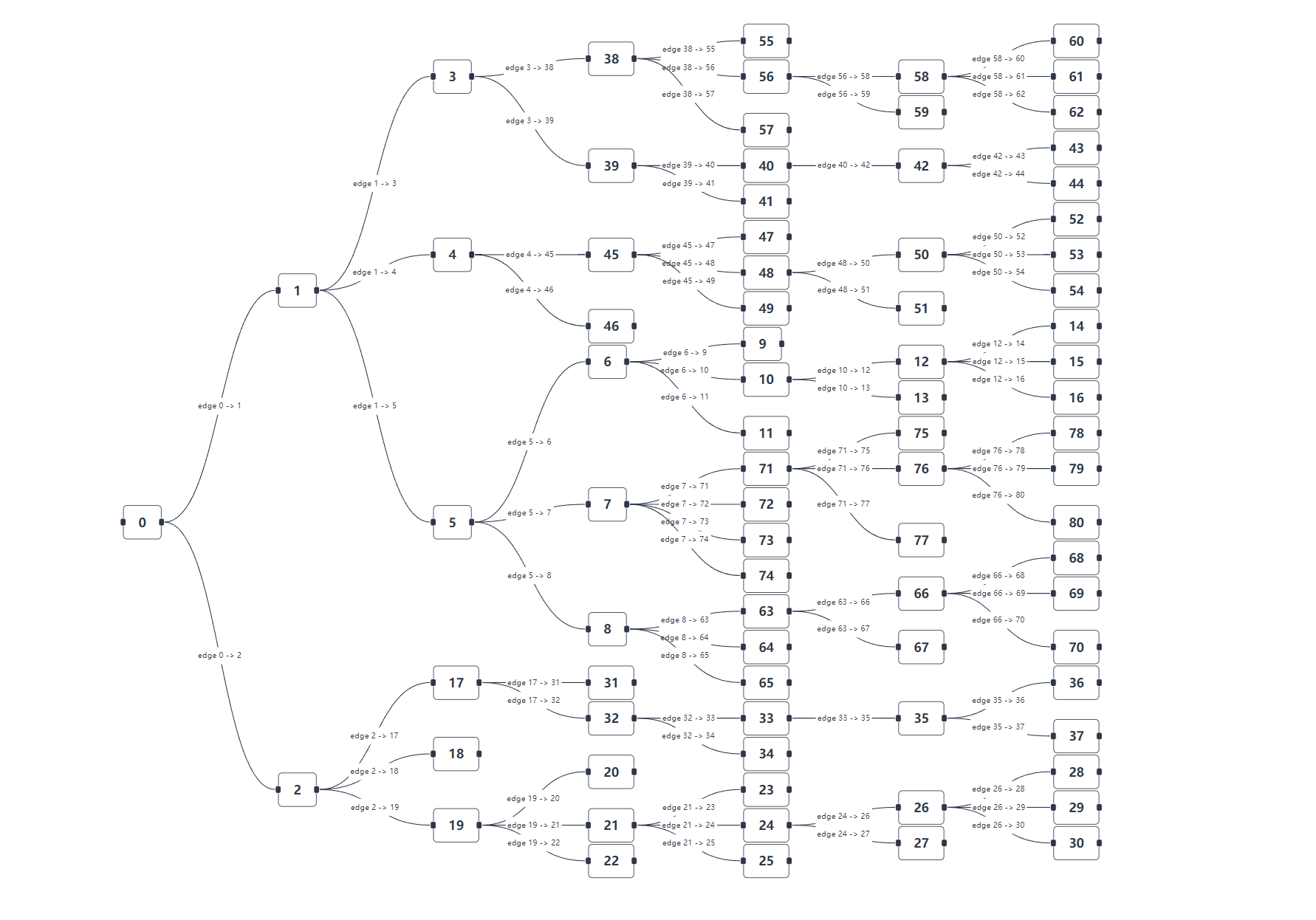
## Directed Graph Diagram: Hierarchical Node-Edge Structure ### Overview The image displays a complex directed graph or tree diagram, structured as a hierarchical flowchart. It originates from a single root node (labeled "0") on the far left and expands rightward through multiple levels of branching. The diagram consists of rectangular nodes containing numerical identifiers and directed edges (arrows) connecting them. Each edge is labeled with text specifying the connection, formatted as "edge [source node] -> [target node]". The overall layout is organized into vertical columns, with each column representing a deeper level in the hierarchy. ### Components/Axes * **Nodes:** Rectangular boxes with rounded corners, each containing a unique integer identifier. The nodes are arranged in vertical columns. * **Edges:** Curved, directed arrows connecting nodes from left to right. Each edge has a text label placed along its path. * **Edge Labels:** Text strings in the format "edge X -> Y", where X is the source node number and Y is the target node number. These labels explicitly define the relationship between connected nodes. * **Spatial Layout:** * **Column 1 (Root):** Contains node `0`. * **Column 2:** Contains nodes `1` and `2`. * **Column 3:** Contains nodes `3`, `4`, `5`, `6`, `7`, `8`, `17`, `18`, `19`. * **Column 4:** Contains a dense set of nodes including `38`, `39`, `45`, `46`, `9`, `10`, `11`, `71`, `72`, `73`, `74`, `63`, `64`, `65`, `31`, `32`, `20`, `21`, `22`. * **Column 5:** Contains nodes such as `55`, `56`, `57`, `40`, `41`, `47`, `48`, `49`, `12`, `13`, `75`, `76`, `77`, `66`, `67`, `33`, `34`, `23`, `24`, `25`. * **Column 6:** Contains nodes like `58`, `59`, `42`, `50`, `51`, `35`, `26`, `27`. * **Column 7 (Leaf Nodes):** The rightmost column contains terminal nodes: `60`, `61`, `62`, `43`, `44`, `52`, `53`, `54`, `14`, `15`, `16`, `78`, `79`, `80`, `68`, `69`, `70`, `36`, `37`, `28`, `29`, `30`. ### Detailed Analysis The graph's structure is defined by the following parent-child relationships, as indicated by the edge labels: * **Root Node `0`** branches to: * Node `1` (via `edge 0 -> 1`) * Node `2` (via `edge 0 -> 2`) * **Node `1`** branches to: * Node `3` (via `edge 1 -> 3`) * Node `4` (via `edge 1 -> 4`) * Node `5` (via `edge 1 -> 5`) * **Node `2`** branches to: * Node `17` (via `edge 2 -> 17`) * Node `18` (via `edge 2 -> 18`) * Node `19` (via `edge 2 -> 19`) * **Sub-branches from Node `3`:** * To Node `38` (via `edge 3 -> 38`) * To Node `39` (via `edge 3 -> 39`) * **Sub-branches from Node `4`:** * To Node `45` (via `edge 4 -> 45`) * To Node `46` (via `edge 4 -> 46`) * **Sub-branches from Node `5`:** * To Node `6` (via `edge 5 -> 6`) * To Node `7` (via `edge 5 -> 7`) * To Node `8` (via `edge 5 -> 8`) * **Sub-branches from Node `6`:** * To Node `9` (via `edge 6 -> 9`) * To Node `10` (via `edge 6 -> 10`) * To Node `11` (via `edge 6 -> 11`) * **Sub-branches from Node `7`:** * To Node `71` (via `edge 7 -> 71`) * To Node `72` (via `edge 7 -> 72`) * To Node `73` (via `edge 7 -> 73`) * To Node `74` (via `edge 7 -> 74`) * **Sub-branches from Node `8`:** * To Node `63` (via `edge 8 -> 63`) * To Node `64` (via `edge 8 -> 64`) * To Node `65` (via `edge 8 -> 65`) * **Sub-branches from Node `17`:** * To Node `31` (via `edge 17 -> 31`) * To Node `32` (via `edge 17 -> 32`) * **Sub-branches from Node `19`:** * To Node `20` (via `edge 19 -> 20`) * To Node `21` (via `edge 19 -> 21`) * To Node `22` (via `edge 19 -> 22`) * **Further branching continues** from nodes like `38`, `39`, `45`, `10`, `12`, `71`, `76`, `63`, `66`, `32`, `33`, `21`, `24`, `26`, etc., ultimately terminating in the leaf nodes listed in Column 7. For example: * Node `38` branches to `55`, `56`, `57`. * Node `56` branches to `58`, `59`. * Node `58` branches to `60`, `61`, `62`. ### Key Observations 1. **Hierarchical Depth:** The graph has a maximum depth of 7 levels (from Node `0` to the leaf nodes). 2. **Branching Factor:** The branching is non-uniform. Some nodes (e.g., `0`, `1`, `5`, `7`) have multiple children (3-4), while others (e.g., many leaf nodes) have none. 3. **Node Numbering:** Node numbers are not assigned sequentially according to their position in the tree. They appear to be arbitrary or based on an external indexing system (e.g., `0`, `1`, `2`, `3`, `4`, `5`, `6`, `7`, `8`, `9`, `10`, `11`, `12`, `13`, `14`, `15`, `16`, `17`, `18`, `19`, `20`, `21`, `22`, `23`, `24`, `25`, `26`, `27`, `28`, `29`, `30`, `31`, `32`, `33`, `34`, `35`, `36`, `37`, `38`, `39`, `40`, `41`, `42`, `43`, `44`, `45`, `46`, `47`, `48`, `49`, `50`, `51`, `52`, `53`, `54`, `55`, `56`, `57`, `58`, `59`, `60`, `61`, `62`, `63`, `64`, `65`, `66`, `67`, `68`, `69`, `70`, `71`, `72`, `73`, `74`, `75`, `76`, `77`, `78`, `79`, `80`). 4. **Edge Label Consistency:** Every visible edge has a corresponding label in the "edge X -> Y" format, providing unambiguous connection data. 5. **Visual Organization:** The layout uses vertical alignment to denote hierarchy levels and curved lines to manage edge crossings, improving readability in dense sections. ### Interpretation This diagram is a formal representation of a **directed acyclic graph (DAG)** or a **tree structure**. It models a system of relationships where each node (except the root) has exactly one incoming edge (from its parent) and can have zero or more outgoing edges (to its children). * **What it represents:** It could depict a workflow, a decision tree, a organizational chart, a data taxonomy, a process flow, or a dependency graph in software or logistics. The numerical labels suggest nodes are identified by an ID rather than a descriptive name. * **Relationships:** The structure clearly defines parent-child relationships and the flow of direction from the root (`0`) outward. The explicit edge labels remove any ambiguity about connections. * **Notable Patterns:** The graph is **not balanced**; some branches are much deeper and more complex than others. For instance, the branch starting with `0 -> 1 -> 5 -> 7 -> 71 -> 76 -> 78` is deep, while `0 -> 2 -> 18` terminates quickly. This suggests an uneven distribution of processes, decisions, or categories within the modeled system. * **Utility:** The primary value of this diagram is in visualizing the complete topology and connectivity of the system. It allows one to trace all possible paths from the root to any terminal point, which is essential for analysis, debugging, or optimization of the underlying process it represents.