## Diagram: Optical Computation with Lenses ### Overview The image is a diagram illustrating an optical computation process using lenses. It shows how an input image is transformed through a series of optical elements, including lenses and intermediate representations, to produce an output image. The diagram highlights the dimensions and parameters involved in the computation. ### Components/Axes * **Axes:** * "computation axis" and "2D input plane" are indicated with arrows, defining the orientation of the diagram. * **Lenses:** Two lenses are depicted, labeled as "F{} lens". * **Input Image:** * A stack of three images, colored red, green, and blue, representing the input channels. * Labeled as "N = nx x ny Cin". * Dimensions are indicated as "nx", "ny", and "Cin". * **Intermediate Representations:** * A grid-like representation between the lenses. * Another grid-like representation after the second lens, labeled with "F{}". * Labeled as "K = k x k Cin". * Dimensions are indicated as "k" and "Cin". * **Output Image:** * A grayscale image on the right side. * Labeled as "M = nx x ny". * Dimensions are indicated as "nx", "ny", and "Cout". * **Parameters:** * "Cin" represents the number of input channels. * "Cout" represents the number of output channels, indicated by "1 ... Cout". * "nx" and "ny" represent the dimensions of the input and output images. * "k" represents the dimensions of the intermediate grid representations. ### Detailed Analysis * **Input Image (N):** The input image is represented as a stack of three color channels (red, green, blue). The dimensions are nx (width), ny (height), and Cin (number of input channels). The equation N = nx x ny Cin suggests that N represents the total number of input elements. * **First Lens (F{} lens):** The first lens transforms the input image into an intermediate representation. A red ray traces the path of light through the lens. * **Intermediate Representation (K):** This representation is a grid with dimensions k x k, and it also incorporates the number of input channels Cin. The equation K = k x k Cin suggests that K represents the total number of elements in this intermediate representation. * **Second Lens (F{} lens):** The second lens performs another transformation on the intermediate representation. * **Output Image (M):** The output image is a grayscale image with dimensions nx x ny. The equation M = nx x ny suggests that M represents the total number of output elements. * **Flow:** Arrows indicate the flow of information from the input image, through the lenses and intermediate representations, to the output image. ### Key Observations * The diagram illustrates an optical computation process where an input image is transformed into an output image using lenses and intermediate representations. * The dimensions and parameters of the input, intermediate, and output representations are clearly labeled. * The lenses are represented as performing some kind of transformation, denoted by "F{}". * The number of input and output channels are represented by Cin and Cout, respectively. ### Interpretation The diagram depicts a conceptual framework for optical computation. The lenses likely represent Fourier transform operations, as suggested by the "F{}" notation. The intermediate representations could be spatial frequency representations of the input image. The process involves transforming the input image into a different domain (e.g., frequency domain), performing some computation in that domain, and then transforming it back to the spatial domain to obtain the output image. The diagram highlights the key parameters and dimensions involved in this process, such as the number of input and output channels, and the dimensions of the intermediate representations. The use of optical elements allows for parallel processing and potentially faster computation compared to traditional digital methods. The transformation "F{}" is applied twice, suggesting a forward and inverse transform pair.

\n ## Diagram: Optical System with 2D Input Plane and Output Volume ### Overview The image depicts a 3D diagram illustrating an optical system that transforms a 2D input plane into a 3D output volume. It appears to model a process akin to a Fourier transform or a similar optical imaging system. The diagram highlights the input plane, two lenses labeled "F{}" lens, an intermediate transformed plane, and the final output volume. Mathematical notations define the dimensions of each plane. ### Components/Axes * **2D input plane:** Located at the bottom-left, representing the initial image. * **Computation axis:** A label pointing to the vertical direction of the input plane. * **F{} lens:** Two lens shapes positioned between the input plane and the intermediate transformed plane. * **Intermediate transformed plane:** A rectangular prism-shaped plane between the lenses. * **Output volume:** Located at the top-right, representing the final transformed image. * **n_x, n_y, n_in:** Dimensions of the input plane. * **k, k_in, c_in, c_out:** Dimensions related to the intermediate and output planes. * **n_x, n_y:** Dimensions of the output volume. * **N = n_x x n_yc_in:** Equation defining the size of the input plane. * **K = k x k c_in:** Equation defining the size of the intermediate transformed plane. * **M = n_x x n_y:** Equation defining the size of the output volume. * **F{}:** Label indicating the function performed by the lenses. * **Arrows:** Red arrows indicate the flow of information through the system. ### Detailed Analysis or Content Details The diagram shows a transformation process. The 2D input plane, with dimensions n_x, n_y, and c_in, is passed through two lenses labeled "F{} lens". These lenses perform a transformation, resulting in an intermediate plane with dimensions k, k, and c_in. The intermediate plane is then transformed into the final output volume with dimensions n_x, n_y, and c_out. The input plane is visually represented as a photograph of a car. The intermediate plane shows a rainbow-like color gradient, suggesting a frequency or spectral representation. The output volume appears as a 3D representation of the input image. The equations provided define the dimensions of each plane: * Input plane size (N): n_x multiplied by n_y multiplied by c_in. * Intermediate plane size (K): k multiplied by k multiplied by c_in. * Output volume size (M): n_x multiplied by n_y. ### Key Observations The diagram illustrates a process that transforms a 2D image into a 3D representation, likely involving a Fourier transform or similar optical imaging technique. The lenses play a crucial role in this transformation, and the intermediate plane represents a frequency-domain representation of the input image. The dimensions of each plane are mathematically defined, providing a quantitative understanding of the transformation process. ### Interpretation This diagram likely represents a simplified model of an optical system used in image processing or computer vision. The "F{}" lenses could represent a Fourier transform lens, which converts a spatial representation of an image into a frequency representation. The intermediate plane then represents the frequency spectrum of the input image. The final output volume represents the reconstructed image in the spatial domain. The use of mathematical notations suggests a focus on the quantitative aspects of the transformation. The diagram could be used to explain the principles of optical imaging, Fourier optics, or related fields. The rainbow-like color gradient in the intermediate plane suggests that the transformation involves a decomposition of the input image into its constituent frequencies. The overall system appears to be designed to capture and process information from a 2D input and represent it in a 3D output space. The diagram is a conceptual illustration rather than a precise engineering blueprint, focusing on the flow of information and the key components involved in the transformation.

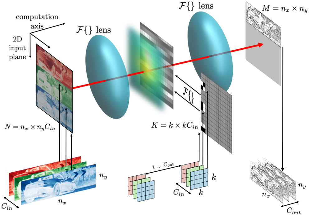
## Technical Diagram: Fourier-Based Convolutional Neural Network Layer ### Overview This image is a technical schematic illustrating the forward pass of a convolutional operation implemented in the Fourier domain, likely within a neural network architecture. It depicts the transformation of a multi-channel input image through frequency-domain processing using lenses (representing Fourier transforms) and multiplication with a kernel, resulting in a transformed output feature map. The diagram emphasizes the mathematical relationships and dimensional transformations involved. ### Components/Axes The diagram is organized into three main spatial regions from left to right, with supporting mathematical notation below. **1. Left Region (Input Stage):** * **Label (Top-Left):** "computation axis" with arrows pointing right and down. * **Label (Top-Left):** "2D input plane". * **Visual Element:** A stack of three colored 2D image planes (red, green, blue channels) representing an input image. * **Dimensional Label (Below input stack):** `N = n_x × n_y C_in`. This denotes the total number of elements in the input tensor, where `n_x` and `n_y` are spatial dimensions and `C_in` is the number of input channels. * **Axis Labels (Bottom-Left):** `C_in` (pointing into the page/depth), `n_x` (horizontal), `n_y` (vertical). **2. Central Region (Processing Stage):** * **Primary Visual Elements:** Two large, blue, elliptical shapes labeled `ℱ{} lens`. These represent Fourier Transform operations. * **Flow:** A red arrow originates from the input plane, passes through the first `ℱ{} lens`, then through a semi-transparent, multi-colored grid (representing the frequency-domain representation of the input), then through a second `ℱ{} lens`, and finally points to the output plane. * **Kernel/Filter (Below central flow):** A 3D grid structure representing a convolutional kernel. * **Dimensional Label:** `K = k × k C_in`. This denotes the kernel's spatial size (`k x k`) and its depth matching the input channels (`C_in`). * **Detailed Kernel View:** A smaller, exploded view shows the kernel's structure with dimensions labeled: `C_in` (depth), `k` (height), `k` (width). An arrow labeled `1 ... C_out` indicates this kernel produces `C_out` output channels. * **Operation Label (Between lenses and kernel):** `ℱ{}` with arrows pointing from the kernel to the central frequency-domain grid, indicating the kernel is also transformed into the frequency domain. **3. Right Region (Output Stage):** * **Visual Element:** A single, grayscale 2D plane representing the output feature map. * **Dimensional Label (Top-Right):** `M = n_x × n_y`. This denotes the spatial dimensions of the output, which match the input's spatial dimensions (`n_x`, `n_y`). * **Axis Labels (Bottom-Right):** `n_x` (horizontal), `n_y` (vertical), `C_out` (pointing into the page/depth). * **Final Output Representation:** A stack of `C_out` grayscale feature maps, showing the result of applying the kernel across all output channels. ### Detailed Analysis The diagram details a specific computational pathway: 1. A multi-channel (`C_in`) input image of size `n_x` by `n_y` is taken. 2. It undergoes a Fourier Transform (`ℱ{}`), visualized as passing through a lens, converting it to the frequency domain. 3. A convolutional kernel of size `k x k x C_in` is also transformed into the frequency domain (`ℱ{}`). 4. The frequency-domain representations of the input and kernel are multiplied element-wise (implied by their convergence at the central grid). 5. The result undergoes an Inverse Fourier Transform (the second `ℱ{} lens`), converting it back to the spatial domain. 6. The final output is a feature map stack with spatial dimensions `n_x` by `n_y` (same as input) and a new depth of `C_out` channels. The red arrow provides a clear visual flow for a single channel/slice through this process. The dimensional labels (`N`, `K`, `M`) explicitly define the size of the data tensors at key stages. ### Key Observations * **Spatial Dimension Preservation:** The output spatial dimensions (`n_x`, `n_y`) are identical to the input's, indicating a "same" convolution (likely achieved via padding in the frequency domain). * **Channel Transformation:** The number of channels changes from `C_in` to `C_out`, controlled by the kernel's fourth dimension. * **Computational Metaphor:** The use of "lenses" for Fourier transforms is a common and effective metaphor in signal processing, implying focusing or transforming the data into a different representation space. * **Kernel Dual Representation:** The kernel is shown both in its spatial form (`k x k x C_in`) and is implied to exist in a frequency-domain form for the multiplication step. ### Interpretation This diagram is a pedagogical illustration of the **Convolution Theorem** applied to deep learning. It demonstrates that convolution in the spatial domain is equivalent to element-wise multiplication in the frequency domain. * **What it Suggests:** The primary purpose is to explain the internal mechanics of a Fourier-based convolutional layer, which can be computationally more efficient than direct spatial convolution for large kernels. It visually breaks down an abstract mathematical operation into a sequence of tangible steps: transform, multiply, inverse transform. * **Relationships:** The elements are causally linked by the red flow arrow. The input and kernel are independent starting points that converge via their frequency-domain representations to produce the output. The `ℱ{} lens` symbols act as the transformative gates between domains. * **Notable Anomalies/Clarifications:** The diagram simplifies the process. In practice, operations like padding, batching, and handling the Hermitian symmetry of real-valued Fourier transforms are necessary but not shown. The "computation axis" label is somewhat abstract but sets the coordinate system for the 2D planes. The color in the central grid likely represents the magnitude or phase of the complex-valued frequency components. **Language Note:** All text in the image is in English, using standard mathematical notation.

## Diagram: Image Transformation Through Optical System ### Overview The diagram illustrates a computational pipeline for image transformation through an optical system, involving Fourier domain processing and feature extraction. It shows the flow of a 2D input image through two lenses (F{}) and intermediate processing stages, resulting in a multi-channel output image. ### Components/Axes 1. **Input Plane (2D Input Plane)** - Dimensions: `N = nx × ny × Cin` - Channels: Red (`C_in`), Green (`C_in`), Blue (`C_in`) - Position: Bottom-left quadrant - Visualization: Color image of a car split into RGB channels 2. **Fourier Plane (F{} Lens)** - Dimensions: `K = k × k × C_in` - Visualization: Blurred grid with intensity variations (green/yellow center) - Position: Center of the diagram - Legend: Gray grid representing spatial frequency domain 3. **Output Plane (M = nx × ny × C_out)** - Dimensions: `M = nx × ny × C_out` - Channels: `C_out` (multiple grayscale feature maps) - Position: Right side of the diagram - Visualization: Edge-detected car images with varying orientations 4. **Computation Axis** - Red arrow connecting input → Fourier plane → output - Indicates data flow direction ### Detailed Analysis - **Input Plane**: - RGB channels (`C_in`) are spatially aligned (`nx × ny` pixels) - Color coding matches standard RGB convention (red/green/blue) - **Fourier Plane**: - Grid structure (`k × k`) suggests convolutional kernel size - Intensity gradient (green/yellow center) implies frequency magnitude representation - **Output Plane**: - `C_out` channels show progressive edge detection (horizontal → vertical → diagonal) - Spatial resolution preserved (`nx × ny`) ### Key Observations 1. **Channel Preservation**: Input channels (`C_in`) are maintained through the Fourier transformation 2. **Feature Multiplication**: Output channels (`C_out`) exceed input channels, indicating feature expansion 3. **Spatial Consistency**: Pixel dimensions (`nx × ny`) remain constant through all stages 4. **Kernel Size**: `k × k` grid in Fourier plane suggests localized frequency analysis ### Interpretation This diagram represents a computational model for image feature extraction using optical system analogies: 1. **First Lens (F{})**: Performs Fourier transform to convert spatial domain image to frequency domain 2. **Fourier Plane Processing**: Implicit filtering occurs in frequency space (green/yellow gradient suggests high-pass filtering) 3. **Second Lens (F{})**: Inverse Fourier transform converts processed frequencies back to spatial domain 4. **Output Channels**: Multiple `C_out` channels demonstrate feature decomposition (e.g., edge detection in different orientations) The system appears to implement a convolutional neural network architecture using optical metaphors, where: - Input plane = Raw image data - Fourier plane = Convolutional filter application in frequency domain - Output plane = Feature maps after non-linear transformation Notable design choices: - Color coding for input channels aids in tracking data flow - Grid visualization in Fourier plane emphasizes frequency localization - Multiple output channels show hierarchical feature extraction