## Line Graphs: Cumulative Variance Explained by PCs (2.5B)
### Overview
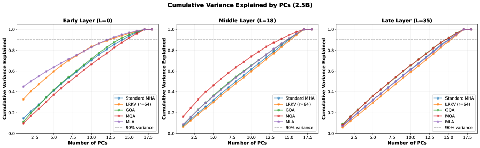
The image contains three line graphs comparing the cumulative variance explained by Principal Components (PCs) across three neural network layers: Early Layer (L=0), Middle Layer (L=18), and Late Layer (L=35). Each graph plots the cumulative variance explained (y-axis) against the number of PCs (x-axis), with five methods represented by distinct colored lines. A gray dashed line indicates the 90% variance threshold.
---
### Components/Axes
- **Title**: "Cumulative Variance Explained by PCs (2.5B)"
- **X-axis**: "Number of PCs" (ranges from 2.5 to 17.5 in increments of 2.5).
- **Y-axis**: "Cumulative Variance Explained" (ranges from 0.0 to 1.0 in increments of 0.2).
- **Legend**:
- **Standard MHA** (blue)
- **LRKV (r=64)** (orange)
- **GQA** (green)
- **MQA** (red)
- **MLA** (purple)
- **90% variance** (gray dashed line).
---
### Detailed Analysis
#### Early Layer (L=0)
- **Standard MHA**: Starts at ~0.15 (2.5 PCs) and rises to ~0.95 (17.5 PCs).
- **LRKV (r=64)**: Starts at ~0.1 (2.5 PCs) and rises to ~0.9 (17.5 PCs).
- **GQA**: Starts at ~0.12 (2.5 PCs) and rises to ~0.92 (17.5 PCs).
- **MQA**: Starts at ~0.1 (2.5 PCs) and rises to ~0.95 (17.5 PCs).
- **MLA**: Starts at ~0.15 (2.5 PCs) and rises to ~0.98 (17.5 PCs).
- **90% threshold**: Reached at ~17.5 PCs for all methods.
#### Middle Layer (L=18)
- **Standard MHA**: Starts at ~0.2 (2.5 PCs) and rises to ~0.98 (17.5 PCs).
- **LRKV (r=64)**: Starts at ~0.15 (2.5 PCs) and rises to ~0.95 (17.5 PCs).
- **GQA**: Starts at ~0.18 (2.5 PCs) and rises to ~0.93 (17.5 PCs).
- **MQA**: Starts at ~0.2 (2.5 PCs) and rises to ~0.97 (17.5 PCs).
- **MLA**: Starts at ~0.25 (2.5 PCs) and rises to ~0.99 (17.5 PCs).
- **90% threshold**: Reached at ~17.5 PCs for all methods.
#### Late Layer (L=35)
- **Standard MHA**: Starts at ~0.3 (2.5 PCs) and rises to ~0.99 (17.5 PCs).
- **LRKV (r=64)**: Starts at ~0.25 (2.5 PCs) and rises to ~0.97 (17.5 PCs).
- **GQA**: Starts at ~0.3 (2.5 PCs) and rises to ~0.95 (17.5 PCs).
- **MQA**: Starts at ~0.3 (2.5 PCs) and rises to ~0.98 (17.5 PCs).
- **MLA**: Starts at ~0.35 (2.5 PCs) and rises to ~1.0 (17.5 PCs).
- **90% threshold**: Reached at ~17.5 PCs for all methods.
---
### Key Observations
1. **Consistent Trends**: All methods show upward-sloping lines, indicating increasing cumulative variance with more PCs.
2. **MLA Dominance**: MLA consistently achieves the highest cumulative variance across all layers, reaching ~1.0 in the Late Layer.
3. **Layer-Specific Differences**:
- Early Layer: Lower starting points (~0.1–0.15) for all methods.
- Middle Layer: Moderate starting points (~0.15–0.25).
- Late Layer: Higher starting points (~0.25–0.35), suggesting greater initial variance capture.
4. **90% Threshold**: All methods reach the 90% variance mark at ~17.5 PCs, regardless of layer.
---
### Interpretation
The graphs demonstrate that **MLA outperforms other methods** in capturing cumulative variance across all layers, particularly in the Late Layer (L=35), where it achieves near-complete variance explanation (~1.0). The **90% threshold** is consistently met at 17.5 PCs, suggesting a standardized benchmark for model performance.
- **Early Layer (L=0)**: Methods require more PCs to explain variance, indicating less efficient feature extraction.
- **Late Layer (L=35)**: Higher initial variance capture (e.g., MLA starts at ~0.35) suggests deeper layers encode more meaningful information.
- **Method Comparisons**:
- **Standard MHA** and **MQA** show similar performance, with MQA slightly outperforming in the Late Layer.
- **LRKV (r=64)** and **GQA** lag behind MLA but remain competitive in the Middle and Late Layers.
The data implies that **MLA’s architecture** is optimized for variance capture, making it suitable for tasks requiring high-dimensional data representation. The consistent 90% threshold across layers highlights the robustness of the PC-based analysis framework.