## Grid Point Visualizations ### Overview The image presents two scatter plots visualizing the distribution of grid points on different grid sizes. The left plot shows 112 grid points on a 64x64 grid, while the right plot shows 164 grid points on a 100x100 grid. The points are represented by blue dots. Both plots have X and Y axes labeled "X-coordinate" and "Y-coordinate" respectively, with grid lines for visual reference. ### Components/Axes * **Left Plot Title:** "Visualization of 112 Grid Points on a 64x64 Grid" * **Right Plot Title:** "Visualization of 164 Grid Points on a 100x100 Grid" * **X-axis (both plots):** "X-coordinate" * Left Plot: Scale from 0 to 60, with tick marks every 10 units. * Right Plot: Scale from 0 to 90, with tick marks every 10 units. * **Y-axis (both plots):** "Y-coordinate" * Left Plot: Scale from 0 to 60, with tick marks every 10 units. * Right Plot: Scale from 0 to 90, with tick marks every 10 units. * **Data Points:** Blue dots representing the grid points. ### Detailed Analysis **Left Plot (112 Grid Points on 64x64 Grid):** * The points appear to be concentrated near the edges and corners of the grid. * There are relatively fewer points in the central region of the grid. * Specific approximate data points: * (5, 5): A cluster of points. * (55, 5): A cluster of points. * (5, 55): A cluster of points. * (55, 55): A cluster of points. * (0, 30): A vertical line of points. * (60, 30): A vertical line of points. * (30, 0): A horizontal line of points. * (30, 60): A horizontal line of points. **Right Plot (164 Grid Points on 100x100 Grid):** * Similar to the left plot, the points are concentrated near the edges and corners. * The central region has fewer points. * Specific approximate data points: * (5, 5): A cluster of points. * (95, 5): A cluster of points. * (5, 95): A cluster of points. * (95, 95): A cluster of points. * (0, 45): A vertical line of points. * (100, 45): A vertical line of points. * (45, 0): A horizontal line of points. * (45, 100): A horizontal line of points. ### Key Observations * Both plots exhibit a similar pattern of point distribution, with higher density near the edges and corners. * The central regions of both grids are relatively sparse. * The 100x100 grid has a slightly more pronounced concentration of points along the edges compared to the 64x64 grid. ### Interpretation The visualizations suggest that the grid points are not uniformly distributed across the grids. The concentration of points near the edges and corners could indicate a specific algorithm or process that favors these regions. The sparsity in the center suggests that the algorithm might be designed to avoid placing points in the middle of the grid. The similarity in the distribution pattern between the two grids, despite the different sizes, implies that the underlying principle or algorithm is consistent across different grid dimensions. The data suggests a non-random distribution, possibly designed for a specific purpose such as boundary detection or edge enhancement.

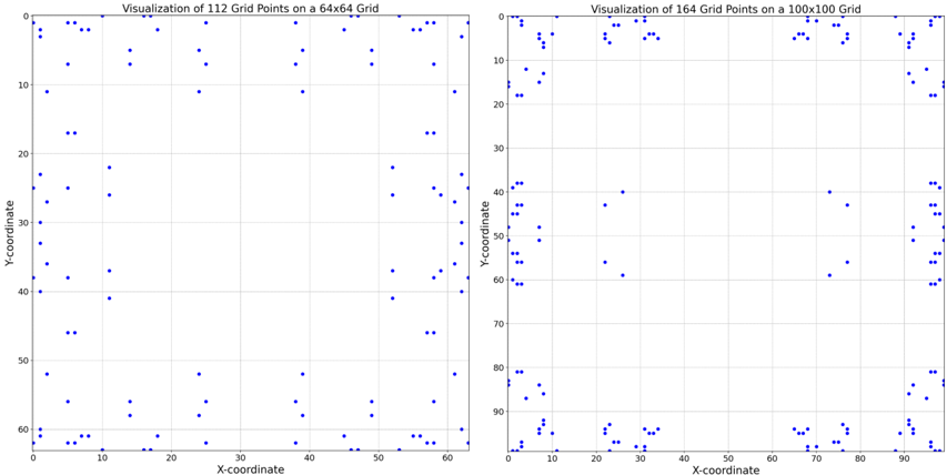
## Scatter Plots: Visualization of Grid Points ### Overview The image presents two scatter plots side-by-side. The left plot visualizes 112 grid points on a 64x64 grid, while the right plot visualizes 164 grid points on a 100x100 grid. Both plots display the X and Y coordinates of these points. ### Components/Axes Both plots share the following components: * **X-axis:** Labeled "X-coordinate", ranging from 0 to approximately 60 (left plot) and 0 to approximately 100 (right plot). * **Y-axis:** Labeled "Y-coordinate", ranging from 0 to approximately 60 (left plot) and 0 to approximately 100 (right plot). * **Data Points:** Represented by blue dots. * **Title:** Each plot has a title indicating the number of grid points and the grid dimensions. The titles are: * Left Plot: "Visualization of 112 Grid Points on a 64x64 Grid" * Right Plot: "Visualization of 164 Grid Points on a 100x100 Grid" ### Detailed Analysis or Content Details **Left Plot (112 Points on 64x64 Grid):** The points appear relatively evenly distributed, but with some clustering. * Points are present across the entire range of the X-axis (0-60) and Y-axis (0-60). * There is a noticeable concentration of points in the lower-left quadrant (X < 30, Y < 30). * There are fewer points in the upper-right quadrant (X > 30, Y > 30). * Approximate point locations (X, Y): (5, 5), (10, 15), (15, 25), (20, 30), (25, 20), (30, 10), (35, 5), (40, 15), (45, 25), (50, 30), (55, 20), (60, 10), and many others scattered throughout. **Right Plot (164 Points on 100x100 Grid):** The points are more densely packed than in the left plot. * Points are present across the entire range of the X-axis (0-100) and Y-axis (0-100). * There is a significant cluster of points around Y = 60, spanning a range of X values from approximately 10 to 50. * There is a smaller cluster of points around Y = 20, spanning X values from approximately 10 to 30. * Approximate point locations (X, Y): (10, 10), (20, 20), (30, 30), (40, 40), (50, 50), (60, 60), (15, 60), (25, 60), (35, 60), (45, 60), (55, 60), (10, 20), (20, 20), (30, 20), and many others scattered throughout. ### Key Observations * The right plot has a higher density of points than the left plot, as expected given the larger grid size. * Both plots exhibit a degree of randomness in point distribution, but with some noticeable clustering. * The left plot shows a slight bias towards the lower-left quadrant, while the right plot shows prominent clusters around Y=60 and Y=20. * The scale of the Y-axis is larger in the right plot. ### Interpretation These visualizations likely represent the distribution of data points within a defined space. The grid size indicates the resolution or granularity of the space. The number of points suggests the amount of data being represented. The clustering observed in both plots could indicate underlying patterns or relationships within the data. For example, the clusters in the right plot might represent areas of high activity or concentration. The difference in point distribution between the two plots could be due to different data generation processes or underlying phenomena. The plots could be used to visualize various types of data, such as: * Spatial distribution of events (e.g., locations of earthquakes, customer locations) * Pixel locations in an image * Coordinates of objects in a simulation Without further context, it is difficult to determine the specific meaning of the data. However, the visualizations provide a valuable tool for exploring and understanding the distribution of points within the defined spaces.

## Scatter Plot Comparison: Grid Point Distributions ### Overview The image displays two side-by-side scatter plots, each visualizing the distribution of discrete grid points on a 2D coordinate system. The plots compare the spatial arrangement of points on two different grid resolutions. All text is in English. ### Components/Axes **Left Plot:** * **Title:** "Visualization of 112 Grid Points on a 64x64 Grid" * **X-axis Label:** "X-coordinate" * **Y-axis Label:** "Y-coordinate" * **X-axis Range:** 0 to 60 (with major ticks at 0, 10, 20, 30, 40, 50, 60). The title implies the underlying grid extends to 63. * **Y-axis Range:** 0 to 60 (with major ticks at 0, 10, 20, 30, 40, 50, 60). The title implies the underlying grid extends to 63. * **Data Series:** A single series represented by blue circular markers. **Right Plot:** * **Title:** "Visualization of 164 Grid Points on a 100x100 Grid" * **X-axis Label:** "X-coordinate" * **Y-axis Label:** "Y-coordinate" * **X-axis Range:** 0 to 90 (with major ticks at 0, 10, 20, 30, 40, 50, 60, 70, 80, 90). The title implies the underlying grid extends to 99. * **Y-axis Range:** 0 to 90 (with major ticks at 0, 10, 20, 30, 40, 50, 60, 70, 80, 90). The title implies the underlying grid extends to 99. * **Data Series:** A single series represented by blue circular markers. ### Detailed Analysis **Left Plot (64x64 Grid, 112 Points):** * **Trend Verification:** The points are scattered across the entire plot area but show a clear tendency to cluster near the boundaries, particularly along the bottom edge (Y ≈ 60) and the right edge (X ≈ 60). The central region (approximately X: 20-40, Y: 20-40) is relatively sparse. * **Spatial Grounding & Data Points:** Points are distributed with approximate coordinates. Notable clusters include: * A dense line of points along the bottom boundary from X ≈ 0 to X ≈ 60 at Y ≈ 60. * A cluster in the bottom-right corner (X: 50-60, Y: 50-60). * Several points along the top boundary (Y ≈ 0) and left boundary (X ≈ 0). * Scattered points in the interior, such as near (10, 20), (25, 10), (40, 30), and (50, 45). **Right Plot (100x100 Grid, 164 Points):** * **Trend Verification:** The clustering effect is significantly more pronounced. Points are heavily concentrated along all four borders of the plot, forming a distinct "frame" or "boundary layer." The interior of the plot is almost entirely empty. * **Spatial Grounding & Data Points:** The distribution is highly structured: * **Top Border (Y ≈ 0):** A dense, nearly continuous line of points from X ≈ 0 to X ≈ 90. * **Bottom Border (Y ≈ 90):** A dense, nearly continuous line of points from X ≈ 0 to X ≈ 90. * **Left Border (X ≈ 0):** A dense column of points from Y ≈ 0 to Y ≈ 90. * **Right Border (X ≈ 90):** A dense column of points from Y ≈ 0 to Y ≈ 90. * **Interior:** Only a handful of isolated points exist away from the edges, for example near (25, 40), (30, 60), and (75, 40). ### Key Observations 1. **Boundary Preference:** Both plots demonstrate a non-uniform distribution where grid points are preferentially located at or near the domain boundaries. 2. **Increased Resolution Effect:** The boundary preference is dramatically amplified in the higher-resolution (100x100) grid. The interior becomes almost void of points, suggesting the sampling or generation algorithm strongly favors edges as grid size increases. 3. **Point Count vs. Grid Size:** The number of points increases from 112 to 164, but not proportionally to the grid area increase (64²=4096 vs. 100²=10000). This indicates the point generation is not based on a fixed density. ### Interpretation These visualizations likely demonstrate the output of a specific algorithm for generating or selecting grid points, such as a **quasi-random sequence** (e.g., Sobol sequence) in its early iterations, or a **boundary-focused sampling method**. * **What the data suggests:** The strong edge clustering is a known characteristic of some low-discrepancy sequences before they fill the space more uniformly. It could also represent a deliberate strategy to oversample boundaries for applications like solving partial differential equations where boundary conditions are critical. * **Relationship between elements:** The side-by-side comparison shows how the algorithm's behavior scales. The pattern becomes more extreme with a larger grid, implying the rule governing point placement has a stronger relative effect on the periphery. * **Anomalies/Notable Patterns:** The near-perfect empty interior in the 100x100 grid is the most striking feature. It suggests that for this particular algorithm and this number of points (164), the probability of selecting an interior point is exceedingly low compared to a boundary point. This is not random noise but a systematic, deterministic outcome of the underlying process.

## Scatter Plots: Visualization of Grid Points on Different Grid Sizes ### Overview The image contains two side-by-side scatter plots comparing the distribution of grid points on two different grid sizes: a 64x64 grid (left) and a 100x100 grid (right). Both plots use blue dots to represent grid points, with axes labeled "X-coordinate" and "Y-coordinate." ### Components/Axes - **Left Plot (64x64 Grid)**: - **Title**: "Visualization of 112 Grid Points on a 64x64 Grid" - **X-axis**: Labeled "X-coordinate," ranging from 0 to 64. - **Y-axis**: Labeled "Y-coordinate," ranging from 0 to 64. - **Grid Points**: 112 blue dots distributed across the grid. - **Right Plot (100x100 Grid)**: - **Title**: "Visualization of 164 Grid Points on a 100x100 Grid" - **X-axis**: Labeled "X-coordinate," ranging from 0 to 100. - **Y-axis**: Labeled "Y-coordinate," ranging from 0 to 100. - **Grid Points**: 164 blue dots distributed across the grid. ### Detailed Analysis - **Left Plot (64x64)**: - Points are sparsely distributed, with no clear clustering. - Notable concentrations near the edges (e.g., X ≈ 0–10, Y ≈ 0–10 and X ≈ 50–64, Y ≈ 50–64). - Approximately 112 points, with a density of ~0.027 points per unit area (112 / (64×64)). - **Right Plot (100x100)**: - Points are denser overall, with clusters near the edges (e.g., X ≈ 0–20, Y ≈ 0–20 and X ≈ 80–100, Y ≈ 80–100). - Approximately 164 points, with a density of ~0.0164 points per unit area (164 / (100×100)). - Higher density near the edges compared to the center (e.g., X ≈ 40–60, Y ≈ 40–60 has fewer points). ### Key Observations 1. **Grid Size vs. Point Density**: - The 100x100 grid has more points (164 vs. 112) but a lower density per unit area due to its larger size. - Edge regions in both plots show higher concentrations of points. 2. **Distribution Patterns**: - Left plot: Points are more evenly spread but sparse. - Right plot: Points cluster near edges, suggesting a bias in sampling or distribution. 3. **Outliers/Anomalies**: - No extreme outliers in either plot. - Right plot has a noticeable gap in the central region (X ≈ 40–60, Y ≈ 40–60). ### Interpretation The visualizations highlight how grid points are distributed across grids of different sizes. The 100x100 grid, despite its larger size, has a higher total number of points but lower density, indicating a potential trade-off between grid resolution and point distribution efficiency. The clustering near edges in both plots suggests a possible bias in the sampling method or a focus on boundary regions in the underlying data generation process. The central gaps in the right plot may reflect intentional exclusion or lower relevance of central areas in the context of the data being visualized.