## Scatter Plot Comparison: Grid Point Distributions
### Overview
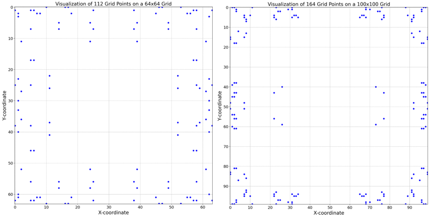
The image displays two side-by-side scatter plots, each visualizing the distribution of discrete grid points on a 2D coordinate system. The plots compare the spatial arrangement of points on two different grid resolutions. All text is in English.
### Components/Axes
**Left Plot:**
* **Title:** "Visualization of 112 Grid Points on a 64x64 Grid"
* **X-axis Label:** "X-coordinate"
* **Y-axis Label:** "Y-coordinate"
* **X-axis Range:** 0 to 60 (with major ticks at 0, 10, 20, 30, 40, 50, 60). The title implies the underlying grid extends to 63.
* **Y-axis Range:** 0 to 60 (with major ticks at 0, 10, 20, 30, 40, 50, 60). The title implies the underlying grid extends to 63.
* **Data Series:** A single series represented by blue circular markers.
**Right Plot:**
* **Title:** "Visualization of 164 Grid Points on a 100x100 Grid"
* **X-axis Label:** "X-coordinate"
* **Y-axis Label:** "Y-coordinate"
* **X-axis Range:** 0 to 90 (with major ticks at 0, 10, 20, 30, 40, 50, 60, 70, 80, 90). The title implies the underlying grid extends to 99.
* **Y-axis Range:** 0 to 90 (with major ticks at 0, 10, 20, 30, 40, 50, 60, 70, 80, 90). The title implies the underlying grid extends to 99.
* **Data Series:** A single series represented by blue circular markers.
### Detailed Analysis
**Left Plot (64x64 Grid, 112 Points):**
* **Trend Verification:** The points are scattered across the entire plot area but show a clear tendency to cluster near the boundaries, particularly along the bottom edge (Y ≈ 60) and the right edge (X ≈ 60). The central region (approximately X: 20-40, Y: 20-40) is relatively sparse.
* **Spatial Grounding & Data Points:** Points are distributed with approximate coordinates. Notable clusters include:
* A dense line of points along the bottom boundary from X ≈ 0 to X ≈ 60 at Y ≈ 60.
* A cluster in the bottom-right corner (X: 50-60, Y: 50-60).
* Several points along the top boundary (Y ≈ 0) and left boundary (X ≈ 0).
* Scattered points in the interior, such as near (10, 20), (25, 10), (40, 30), and (50, 45).
**Right Plot (100x100 Grid, 164 Points):**
* **Trend Verification:** The clustering effect is significantly more pronounced. Points are heavily concentrated along all four borders of the plot, forming a distinct "frame" or "boundary layer." The interior of the plot is almost entirely empty.
* **Spatial Grounding & Data Points:** The distribution is highly structured:
* **Top Border (Y ≈ 0):** A dense, nearly continuous line of points from X ≈ 0 to X ≈ 90.
* **Bottom Border (Y ≈ 90):** A dense, nearly continuous line of points from X ≈ 0 to X ≈ 90.
* **Left Border (X ≈ 0):** A dense column of points from Y ≈ 0 to Y ≈ 90.
* **Right Border (X ≈ 90):** A dense column of points from Y ≈ 0 to Y ≈ 90.
* **Interior:** Only a handful of isolated points exist away from the edges, for example near (25, 40), (30, 60), and (75, 40).
### Key Observations
1. **Boundary Preference:** Both plots demonstrate a non-uniform distribution where grid points are preferentially located at or near the domain boundaries.
2. **Increased Resolution Effect:** The boundary preference is dramatically amplified in the higher-resolution (100x100) grid. The interior becomes almost void of points, suggesting the sampling or generation algorithm strongly favors edges as grid size increases.
3. **Point Count vs. Grid Size:** The number of points increases from 112 to 164, but not proportionally to the grid area increase (64²=4096 vs. 100²=10000). This indicates the point generation is not based on a fixed density.
### Interpretation
These visualizations likely demonstrate the output of a specific algorithm for generating or selecting grid points, such as a **quasi-random sequence** (e.g., Sobol sequence) in its early iterations, or a **boundary-focused sampling method**.
* **What the data suggests:** The strong edge clustering is a known characteristic of some low-discrepancy sequences before they fill the space more uniformly. It could also represent a deliberate strategy to oversample boundaries for applications like solving partial differential equations where boundary conditions are critical.
* **Relationship between elements:** The side-by-side comparison shows how the algorithm's behavior scales. The pattern becomes more extreme with a larger grid, implying the rule governing point placement has a stronger relative effect on the periphery.
* **Anomalies/Notable Patterns:** The near-perfect empty interior in the 100x100 grid is the most striking feature. It suggests that for this particular algorithm and this number of points (164), the probability of selecting an interior point is exceedingly low compared to a boundary point. This is not random noise but a systematic, deterministic outcome of the underlying process.