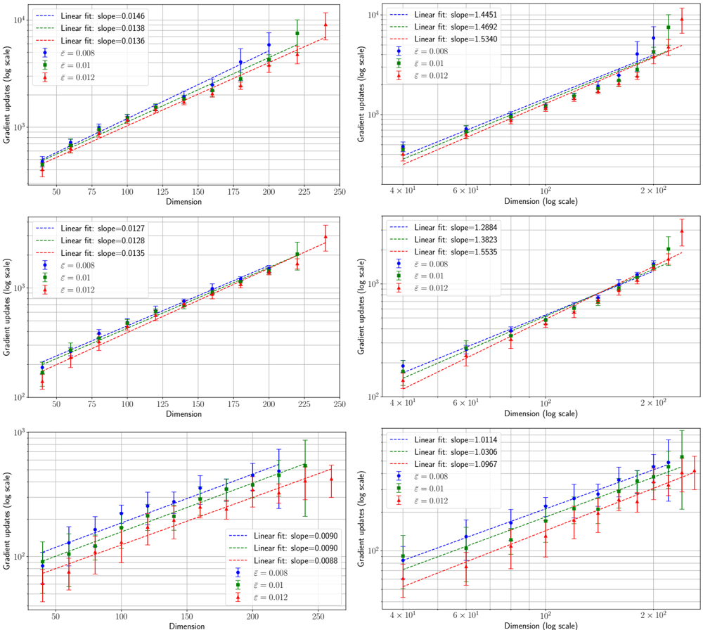
## Scatter Plots with Linear Fits: Gradient Updates vs. Dimension ### Overview The image contains six individual scatter plots arranged in a 3x2 grid. Each plot displays the relationship between "Gradient updates (log scale)" on the y-axis and "Dimension" on the x-axis for three different values of a parameter denoted by epsilon (ε). Each data series includes error bars and is fitted with a linear regression line. The plots appear to compare scaling behaviors under different conditions or datasets. ### Components/Axes * **Plot Layout:** 3 rows x 2 columns. * **Y-axis (All Plots):** Label is "Gradient updates (log scale)". The scale is logarithmic (base 10), with major ticks at powers of 10 (e.g., 10², 10³, 10⁴). * **X-axis (Left Column Plots):** Label is "Dimension". The scale is linear, with major ticks typically at 50, 75, 100, 125, 150, 175, 200, 225, 250. * **X-axis (Right Column Plots):** Label is "Dimension (log scale)". The scale is logarithmic, with major ticks at 4x10¹, 6x10¹, 10², 2x10². * **Legend (Present in all plots):** Located in the top-left corner of each plot area. It contains: * Three entries for linear fit lines, each with a dashed line style and a specific color, reporting the slope. * Three entries for data series markers, each with a specific color and error bar style, reporting the ε value. * **Data Series & Colors:** * **Blue circles with error bars:** ε = 0.008 * **Green squares with error bars:** ε = 0.01 * **Red triangles with error bars:** ε = 0.012 * **Linear Fit Lines (Dashed):** * **Blue dashed line:** Corresponds to the fit for the ε = 0.008 series. * **Green dashed line:** Corresponds to the fit for the ε = 0.01 series. * **Red dashed line:** Corresponds to the fit for the ε = 0.012 series. ### Detailed Analysis **Plot 1 (Top-Left):** * **X-axis:** Linear scale (50-250). * **Linear Fit Slopes:** * Blue (ε=0.008): slope=0.0146 * Green (ε=0.01): slope=0.0138 * Red (ε=0.012): slope=0.0136 * **Trend:** All three series show a clear upward trend. The number of gradient updates increases with dimension. The slopes are very close, with the smallest ε (0.008) having a slightly steeper slope. **Plot 2 (Top-Right):** * **X-axis:** Log scale (~40 to ~250). * **Linear Fit Slopes:** * Blue (ε=0.008): slope=1.4451 * Green (ε=0.01): slope=1.4692 * Red (ε=0.012): slope=1.5340 * **Trend:** All series show a strong upward trend on the log-log plot, indicating a power-law relationship. The slopes are all greater than 1, suggesting a super-linear scaling. Here, the largest ε (0.012) has the steepest slope. **Plot 3 (Middle-Left):** * **X-axis:** Linear scale (50-250). * **Linear Fit Slopes:** * Blue (ε=0.008): slope=0.0127 * Green (ε=0.01): slope=0.0128 * Red (ε=0.012): slope=0.0135 * **Trend:** Upward trend. Slopes are very similar, with the largest ε (0.012) having a marginally higher slope. **Plot 4 (Middle-Right):** * **X-axis:** Log scale (~40 to ~250). * **Linear Fit Slopes:** * Blue (ε=0.008): slope=1.2884 * Green (ε=0.01): slope=1.3823 * Red (ε=0.012): slope=1.5535 * **Trend:** Strong upward trend on log-log plot. Slopes are all >1, indicating super-linear scaling. The slope increases noticeably with ε. **Plot 5 (Bottom-Left):** * **X-axis:** Linear scale (50-250). * **Linear Fit Slopes:** * Blue (ε=0.008): slope=0.0090 * Green (ε=0.01): slope=0.0090 * Red (ε=0.012): slope=0.0088 * **Trend:** Upward trend. Slopes are nearly identical for ε=0.008 and ε=0.01, and slightly lower for ε=0.012. The overall slopes are lower than in Plots 1 and 3. **Plot 6 (Bottom-Right):** * **X-axis:** Log scale (~40 to ~250). * **Linear Fit Slopes:** * Blue (ε=0.008): slope=1.0114 * Green (ε=0.01): slope=1.0306 * Red (ε=0.012): slope=1.0967 * **Trend:** Upward trend on log-log plot. Slopes are very close to 1, suggesting an approximately linear relationship between log(Gradient updates) and log(Dimension), which corresponds to a power-law relationship with an exponent near 1. The slope increases slightly with ε. ### Key Observations 1. **Consistent Positive Correlation:** In all six plots, the number of gradient updates increases as the dimension increases. 2. **Effect of Axis Scale:** The left column (linear x-axis) shows roughly linear relationships. The right column (log x-axis) shows linear relationships on the log-log plot, indicating power-law scaling (Gradient updates ∝ Dimension^k). 3. **Slope Variation with ε:** The relationship between the fit slope and ε is not consistent across all plots. In some (e.g., Top-Right, Middle-Right), slope increases with ε. In others (e.g., Top-Left, Bottom-Left), the relationship is weaker or reversed. 4. **Magnitude of Slopes:** The slopes in the right-column (log-scale) plots are orders of magnitude larger than those in the left-column plots, which is expected due to the different x-axis scaling. The slopes in the bottom row plots are generally smaller than those in the top and middle rows. 5. **Error Bars:** The error bars (uncertainty) appear relatively consistent across dimensions within each plot but vary in size between different plots. ### Interpretation This set of plots likely comes from an empirical study in machine learning or optimization, investigating how the computational cost (measured in gradient updates) scales with the problem dimensionality under different privacy or noise regimes (parameterized by ε). * **Scaling Laws:** The data demonstrates that gradient update cost scales super-linearly with dimension in most scenarios (slopes >1 on log-log plots). The exact scaling exponent (the slope on the log-log plot) varies, suggesting it depends on the specific experimental setup or dataset represented by each of the six plots. * **Role of Epsilon (ε):** The parameter ε, often associated with the privacy budget in differential privacy, influences the scaling. A larger ε (less privacy/less noise) sometimes leads to a steeper scaling (higher slope), meaning the cost grows faster with dimension. However, this effect is not universal across all six conditions, indicating that the relationship between privacy budget and computational scaling is complex and context-dependent. * **Practical Implication:** The plots provide quantitative evidence for the "cost of scale." As the dimensionality of a problem increases, the number of required gradient updates grows according to a power law. This has direct implications for the feasibility and resource requirements of training high-dimensional models, especially under constraints like differential privacy. The variation across the six plots suggests that algorithmic choices or data characteristics significantly modulate this scaling behavior.