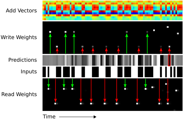
## Diagram: Neural Network Memory Operations Over Time ### Overview The image is a multi-panel technical diagram illustrating the internal operations of a neural network model, likely a memory-augmented or recurrent architecture, over a sequence of time steps. It visualizes the flow of data, weight updates, and predictions. The diagram is composed of five horizontally stacked panels, each representing a different component or data stream, aligned along a common time axis. ### Components/Axes The diagram is segmented into five distinct horizontal panels, each labeled on the left side. From top to bottom: 1. **Add Vectors**: A heatmap visualization. 2. **Write Weights**: A sparse matrix with directional arrows. 3. **Predictions**: A grayscale intensity bar. 4. **Inputs**: A binary (black and white) sequence. 5. **Read Weights**: A sparse matrix with directional arrows. A single **Time** axis runs along the bottom of the entire diagram, with an arrow pointing to the right (`→`), indicating that the horizontal dimension represents progression through time for all panels. ### Detailed Analysis **Panel 1: Add Vectors** * **Visual**: A dense heatmap with a grid structure. The color gradient ranges from deep blue (cool) through cyan, yellow, and orange to deep red (hot). * **Interpretation**: This likely represents the accumulation or summation of activation vectors or memory content over time. The color intensity indicates the magnitude of values, with red being the highest and blue the lowest. The pattern shows vertical bands of similar color, suggesting that certain time steps have consistently high or low summed values. **Panel 2: Write Weights** * **Visual**: A black background with sparse white squares. Green arrows point upward (`↑`) to some white squares, and red arrows point downward (`↓`) to others. * **Spatial Grounding**: The white squares are scattered across the panel. The green and red arrows are interspersed along the time axis. * **Interpretation**: This panel visualizes the "write" operations to a memory matrix. The white squares represent memory locations being accessed. The green upward arrows likely indicate an increase or positive update to the weight at that location and time, while the red downward arrows indicate a decrease or negative update. **Panel 3: Predictions** * **Visual**: A continuous horizontal bar composed of vertical grayscale stripes. The shades range from black to white. * **Trend Verification**: The bar shows a dynamic pattern of dark and light bands, indicating that the model's predicted output values fluctuate over time. There is no single monotonic trend; instead, it shows periods of high confidence (bright white) and low confidence or different class predictions (dark gray/black). **Panel 4: Inputs** * **Visual**: A binary sequence of solid black and white vertical bars of varying widths. * **Interpretation**: This represents the raw input data stream fed into the model over time. Black and white likely correspond to binary states (e.g., 0 and 1, or off and on). The varying widths indicate that some input states persist for multiple time steps. **Panel 5: Read Weights** * **Visual**: Similar to the "Write Weights" panel, with a black background and sparse white squares. Here, green arrows point downward (`↓`) and red arrows point downward (`↓`) as well, but their placement differs from the "Write Weights" panel. * **Spatial Grounding & Cross-Reference**: The white squares (memory locations accessed for reading) are in different positions compared to the "Write Weights" panel. The green and red arrows here both point downward, which may signify a different operation (e.g., reading vs. writing) or a different type of read (e.g., attending to vs. suppressing). * **Interpretation**: This shows the "read" operations from memory. The model is attending to specific memory locations (white squares) at specific times to retrieve information for making predictions. The color of the arrows (green/red) may correlate with the type of information retrieved or its effect on the prediction. ### Key Observations 1. **Temporal Alignment**: All panels are perfectly aligned vertically, meaning a single column represents a single time step. This allows for cross-panel analysis (e.g., seeing what the input was when a specific memory location was written to). 2. **Sparse Memory Access**: Both "Write Weights" and "Read Weights" panels show that only a few memory locations (white squares) are active at any given time step, indicating a sparse access pattern. 3. **Correlation Between Panels**: There is a visible, though complex, relationship between the panels. For instance, specific patterns in the "Inputs" sequence appear to trigger "Write" operations (green/red arrows in the second panel) and later influence "Read" operations (fifth panel), which in turn correlate with changes in the "Predictions" bar. 4. **Color Coding Consistency**: Green and red are used consistently in the weight panels to denote opposing operations or effects (e.g., increase/decrease, excite/inhibit). ### Interpretation This diagram provides a "look under the hood" of a neural network's memory mechanism. It demonstrates how the model processes a sequential input (`Inputs`), dynamically updates its internal memory (`Write Weights`), and then uses that memory (`Read Weights`) to generate time-step-specific `Predictions`. The `Add Vectors` heatmap likely shows the net effect of these read/write operations on the model's internal state. The key takeaway is the model's dynamic and selective use of memory. It doesn't store or recall everything; it writes to and reads from specific memory slots at specific times, guided by the input data. The fluctuating `Predictions` bar shows the direct output of this complex, memory-augmented processing. The diagram effectively argues that the model's behavior is not a simple feed-forward function but a stateful process where past inputs (stored via writes) actively influence current outputs (via reads). The sparse access pattern suggests an efficient use of memory resources, focusing only on relevant information.