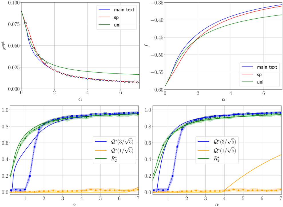
## Four Line Charts: Comparative Analysis of Algorithms ### Overview The image presents four line charts arranged in a 2x2 grid, comparing the performance of different algorithms across a range of alpha values. The top-left chart displays epsilon-opt values, the top-right chart displays 'f' values, and the bottom two charts display performance metrics Q*(3/√5), Q*(1/√5), and R*_2. The bottom two charts appear to be variations of the same data, possibly representing different experimental conditions or perspectives. ### Components/Axes **Top-Left Chart:** * **Title:** Implicit, represents epsilon-opt values. * **X-axis:** α (Alpha), ranging from 0 to 7. * **Y-axis:** ε^opt, ranging from 0.000 to 0.100, with increments of 0.025. * **Legend (Top-Right):** * Blue line: "main text" * Red line: "sp" * Green line: "uni" **Top-Right Chart:** * **Title:** Implicit, represents 'f' values. * **X-axis:** α (Alpha), ranging from 0 to 6. * **Y-axis:** f, ranging from -0.60 to -0.35, with increments of 0.05. * **Legend (Bottom-Right):** * Blue line: "main text" * Red line: "sp" * Green line: "uni" **Bottom-Left Chart:** * **Title:** Implicit, represents performance metrics. * **X-axis:** α (Alpha), ranging from 0 to 7. * **Y-axis:** Values ranging from 0.0 to 1.0, with increments of 0.2. * **Legend (Right):** * Blue line: "Q*(3/√5)" * Orange line: "Q*(1/√5)" * Green line: "R*_2" **Bottom-Right Chart:** * **Title:** Implicit, represents performance metrics. * **X-axis:** α (Alpha), ranging from 0 to 7. * **Y-axis:** Values ranging from 0.0 to 1.0, with increments of 0.2. * **Legend (Right):** * Blue line: "Q*(3/√5)" * Orange line: "Q*(1/√5)" * Green line: "R*_2" ### Detailed Analysis **Top-Left Chart (ε^opt vs. α):** * **"main text" (Blue):** Starts at approximately 0.05, decreases rapidly, and plateaus around 0.01 after α = 2. * α = 0: ε^opt ≈ 0.05 * α = 2: ε^opt ≈ 0.015 * α = 6: ε^opt ≈ 0.01 * **"sp" (Red):** Starts at approximately 0.08, decreases rapidly, and plateaus around 0.01 after α = 2. * α = 0: ε^opt ≈ 0.08 * α = 2: ε^opt ≈ 0.015 * α = 6: ε^opt ≈ 0.01 * **"uni" (Green):** Starts at approximately 0.08, decreases gradually, and plateaus around 0.02 after α = 4. * α = 0: ε^opt ≈ 0.08 * α = 2: ε^opt ≈ 0.03 * α = 6: ε^opt ≈ 0.02 **Top-Right Chart (f vs. α):** * **"main text" (Blue):** Starts at approximately -0.60, increases rapidly, and plateaus around -0.38 after α = 4. * α = 0: f ≈ -0.60 * α = 2: f ≈ -0.45 * α = 6: f ≈ -0.38 * **"sp" (Red):** Starts at approximately -0.60, increases rapidly, and plateaus around -0.40 after α = 4. * α = 0: f ≈ -0.60 * α = 2: f ≈ -0.47 * α = 6: f ≈ -0.40 * **"uni" (Green):** Starts at approximately -0.60, increases rapidly, and plateaus around -0.42 after α = 4. * α = 0: f ≈ -0.60 * α = 2: f ≈ -0.49 * α = 6: f ≈ -0.42 **Bottom-Left Chart (Performance Metrics vs. α):** * **"Q*(3/√5)" (Blue):** Starts at approximately 0.0, jumps to approximately 0.8 at α = 1, and plateaus around 0.95 after α = 3. * α = 0: Value ≈ 0.0 * α = 1: Value ≈ 0.8 * α = 3: Value ≈ 0.95 * α = 7: Value ≈ 0.95 * **"Q*(1/√5)" (Orange):** Remains near 0.0 across all alpha values. * α = 0: Value ≈ 0.0 * α = 7: Value ≈ 0.0 * **"R*_2" (Green):** Starts at approximately 0.2, increases rapidly, and plateaus around 0.95 after α = 3. * α = 0: Value ≈ 0.2 * α = 2: Value ≈ 0.8 * α = 3: Value ≈ 0.95 * α = 7: Value ≈ 0.95 **Bottom-Right Chart (Performance Metrics vs. α):** * **"Q*(3/√5)" (Blue):** Starts at approximately 0.0, jumps to approximately 0.8 at α = 1, and plateaus around 0.95 after α = 3. * α = 0: Value ≈ 0.0 * α = 1: Value ≈ 0.8 * α = 3: Value ≈ 0.95 * α = 7: Value ≈ 0.95 * **"Q*(1/√5)" (Orange):** Starts at approximately 0.0, increases gradually, reaching approximately 0.45 at α = 7. * α = 0: Value ≈ 0.0 * α = 7: Value ≈ 0.45 * **"R*_2" (Green):** Starts at approximately 0.2, increases rapidly, and plateaus around 0.95 after α = 3. * α = 0: Value ≈ 0.2 * α = 2: Value ≈ 0.8 * α = 3: Value ≈ 0.95 * α = 7: Value ≈ 0.95 ### Key Observations * In the top-left chart, "main text" and "sp" algorithms have similar performance, achieving lower epsilon-opt values compared to "uni" as alpha increases. * In the top-right chart, all three algorithms ("main text", "sp", and "uni") converge to similar 'f' values as alpha increases. * In the bottom-left chart, "Q*(3/√5)" and "R*_2" metrics show a significant jump in performance around α = 1, while "Q*(1/√5)" remains consistently low. * In the bottom-right chart, "Q*(3/√5)" and "R*_2" metrics show a significant jump in performance around α = 1, while "Q*(1/√5)" increases gradually. * The bottom-left and bottom-right charts differ primarily in the behavior of the "Q*(1/√5)" metric, which remains near zero in the bottom-left chart but increases gradually in the bottom-right chart. ### Interpretation The charts provide a comparative analysis of different algorithms ("main text", "sp", and "uni") and their performance metrics ("Q*(3/√5)", "Q*(1/√5)", and "R*_2") across varying alpha values. The top charts suggest that "main text" and "sp" algorithms are more effective in minimizing epsilon-opt compared to "uni". The bottom charts indicate that "Q*(3/√5)" and "R*_2" metrics exhibit a threshold behavior, with a significant performance jump around α = 1. The difference in "Q*(1/√5)" behavior between the bottom-left and bottom-right charts suggests that this metric is sensitive to specific experimental conditions or parameter settings. The data suggests that the choice of algorithm and alpha value significantly impacts performance, and the optimal configuration depends on the specific metric being optimized.

## Chart Type: Multi-panel Scientific Data Visualization ### Overview This image consists of four separate subplots arranged in a 2x2 grid. The charts illustrate the relationship between a parameter $\alpha$ (on the horizontal axis) and various performance metrics or physical quantities (on the vertical axes). The data appears to compare theoretical predictions (solid lines) with numerical simulations (dashed lines and markers). ### Components/Axes #### Global Features * **X-axis (all plots):** Labeled $\alpha$, ranging from 0 to 7. * **Grid:** All plots feature a light gray background grid for easier value estimation. #### Top-Left Plot: Error Metric * **Y-axis:** Labeled $\epsilon^{opt}$, ranging from 0.000 to 0.100. * **Legend (Top-Right):** * **Blue line:** `main text` * **Red line:** `sp` * **Green line:** `uni` * **Markers:** White circles with black outlines and vertical error bars follow the blue/red lines. #### Top-Right Plot: Potential/Free Energy Metric * **Y-axis:** Labeled $f$, ranging from -0.60 to -0.35. * **Legend (Bottom-Right):** * **Blue line:** `main text` * **Red line:** `sp` * **Green line:** `uni` #### Bottom-Left Plot: Order Parameters / Overlaps (Set A) * **Y-axis:** Unlabeled, ranging from 0.0 to 1.0. * **Legend (Center-Right):** * **Blue line:** $\mathcal{Q}^*(3/\sqrt{5})$ * **Yellow line:** $\mathcal{Q}^*(1/\sqrt{5})$ * **Green line:** $R_2^*$ * **Markers/Shading:** * Blue dashed line with square markers and blue shaded uncertainty region. * Green dashed line with triangle markers and green shaded uncertainty region. * Yellow dashed line with circle markers and yellow shaded uncertainty region. #### Bottom-Right Plot: Order Parameters / Overlaps (Set B) * **Y-axis:** Unlabeled, ranging from 0.0 to 1.0. * **Legend (Center-Right):** Same as Bottom-Left. * **Markers/Shading:** Same as Bottom-Left. --- ### Detailed Analysis #### Top-Left: $\epsilon^{opt}$ vs $\alpha$ * **Trend:** All three series show a monotonic decrease as $\alpha$ increases. * **Green line (uni):** Slopes downward gradually. At $\alpha=0$, $\epsilon^{opt} \approx 0.09$. At $\alpha=7$, $\epsilon^{opt} \approx 0.018$. * **Red line (sp) & Blue line (main text):** These two are nearly identical. They drop much faster than the green line. At $\alpha=2$, $\epsilon^{opt} \approx 0.02$. At $\alpha=7$, $\epsilon^{opt} \approx 0.008$. * **Markers:** The experimental data points (white circles) align closely with the `sp` and `main text` theoretical lines. #### Top-Right: $f$ vs $\alpha$ * **Trend:** All three series show a monotonic increase as $\alpha$ increases. * **Starting Point:** All lines originate from approximately $f \approx -0.59$ at $\alpha=0$. * **Blue line (main text):** Shows the steepest increase, reaching $\approx -0.36$ at $\alpha=7$. * **Red line (sp):** Slightly below the blue line, reaching $\approx -0.37$ at $\alpha=7$. * **Green line (uni):** The shallowest increase, reaching $\approx -0.385$ at $\alpha=7$. #### Bottom-Left: Overlap Metrics * **Green Series ($R_2^*$):** The solid line rises quickly from $\approx 0.2$ at $\alpha=0$ to a plateau of $\approx 0.95$ by $\alpha=4$. The dashed line with triangles follows this trend closely. * **Blue Series ($\mathcal{Q}^*(3/\sqrt{5})$):** * **Solid line:** Rises sharply from 0 starting at $\alpha \approx 0.2$, crossing the green line at $\alpha \approx 1.5$. * **Dashed line (squares):** Stays near 0 until $\alpha \approx 1.2$, then exhibits a discontinuous "jump" to meet the solid line by $\alpha \approx 2$. * **Yellow Series ($\mathcal{Q}^*(1/\sqrt{5})$):** The solid line remains at 0 until $\alpha \approx 6.5$, where it begins a sharp rise. The dashed line (circles) remains near 0 for the entire range shown. #### Bottom-Right: Overlap Metrics (Alternative Condition) * **Green and Blue Series:** Behave very similarly to the Bottom-Left plot. The blue dashed line jump occurs slightly later, around $\alpha \approx 1.5$. * **Yellow Series ($\mathcal{Q}^*(1/\sqrt{5})$):** * **Solid line:** Remains at 0 until $\alpha \approx 4.0$, then rises linearly to reach $\approx 0.45$ at $\alpha=7$. * **Dashed line (circles):** Remains near 0 for the entire range, failing to follow the theoretical rise. --- ### Key Observations 1. **Efficiency Gains:** In the top-left plot, the `main text` and `sp` methods significantly outperform the `uni` method, achieving lower error ($\epsilon^{opt}$) for the same value of $\alpha$. 2. **Phase Transitions:** The bottom plots show clear evidence of phase transitions. The sharp jumps in the dashed lines (empirical data) compared to the smoother or earlier rises in solid lines (theoretical equilibrium) suggest the presence of metastable states and "spinodal" points. 3. **Discrepancy in Yellow Series:** In both bottom plots, the empirical yellow data (circles) fails to track the theoretical rise (solid line) within the observed range of $\alpha$, suggesting a very high barrier to entry for that specific state or a much later transition point in practice. --- ### Interpretation The data likely describes a system in statistical mechanics or high-dimensional inference (such as a neural network or compressed sensing). * **$\alpha$** typically represents "sample complexity" or the ratio of data points to dimensions. * **$\epsilon^{opt}$** is likely an optimality gap or generalization error. * **$f$** likely represents the free energy of the system. * **The bottom plots** show "order parameters" or overlaps between the system's state and a ground truth. The "jump" in the blue dashed line in the bottom panels is a classic signature of a **first-order phase transition**. The theoretical solid line represents the global minimum of the free energy, while the dashed line represents the path taken by a local algorithm (like gradient descent or approximate message passing). The algorithm stays "trapped" in a poor state (near 0) until $\alpha$ is large enough to collapse the barrier, at which point it jumps to the "good" state (near 1). The difference between the bottom-left and bottom-right plots (specifically the yellow line) suggests that the right-hand scenario has parameters that make the second "good" state ($\mathcal{Q}^*(1/\sqrt{5})$) theoretically accessible much earlier, though still not reached by the simulation.

## Charts: Parameter Dependence of Quantities ### Overview The image contains four separate charts, arranged in a 2x2 grid, depicting the relationship between a parameter α (on the x-axis) and various quantities (on the y-axis). Each chart displays multiple curves, each representing a different model or condition ("main text", "sp", "uni", Q*(3/√5), Q*(1/√5), R₂*). The charts appear to be exploring the behavior of these quantities as α varies. ### Components/Axes All four charts share the same x-axis label: "α". The y-axis labels differ for each chart: * Top-Left: "ω_0" * Top-Right: "f" * Bottom-Left: (No explicit label, but values range from 0 to 1) * Bottom-Right: (No explicit label, but values range from 0 to 1) The legend is positioned in the top-right corner of each chart and contains the following labels with corresponding colors: * "main text" - Blue * "sp" - Red * "uni" - Green * Q*(3/√5) - Dark Blue * Q*(1/√5) - Orange * R₂* - Green ### Detailed Analysis or Content Details **Top-Left Chart (ω_0 vs. α):** * The blue line ("main text") starts at approximately ω_0 = 0.075 at α = 0 and decreases rapidly, approaching 0 as α increases. * The red line ("sp") starts at approximately ω_0 = 0.065 at α = 0 and decreases more slowly than the blue line, also approaching 0 as α increases. * The green line ("uni") starts at approximately ω_0 = 0.03 at α = 0 and decreases even more slowly than the red line, approaching 0 as α increases. * All three lines exhibit a decreasing trend. **Top-Right Chart (f vs. α):** * The blue line ("main text") starts at approximately f = -0.55 at α = 0 and increases rapidly, approaching approximately f = -0.35 as α increases. * The red line ("sp") starts at approximately f = -0.50 at α = 0 and increases more slowly than the blue line, approaching approximately f = -0.40 as α increases. * The green line ("uni") starts at approximately f = -0.45 at α = 0 and increases at a constant rate, approaching approximately f = -0.35 as α increases. * All three lines exhibit an increasing trend. **Bottom-Left Chart (Unlabeled vs. α):** * The dark blue line (Q*(3/√5)) starts at approximately 0 at α = 0 and increases rapidly, reaching approximately 0.8 at α = 2, and then plateaus around 0.95. * The orange line (Q*(1/√5)) remains close to 0 for α values up to approximately 3, then increases slowly to around 0.2. * The green line (R₂*) starts at approximately 0 at α = 0 and increases rapidly, reaching approximately 0.8 at α = 2, and then plateaus around 0.95. * The dark blue and green lines show a similar trend, while the orange line remains significantly lower. **Bottom-Right Chart (Unlabeled vs. α):** * The dark blue line (Q*(3/√5)) starts at approximately 0 at α = 0 and increases rapidly, reaching approximately 0.8 at α = 2, and then plateaus around 0.95. * The orange line (Q*(1/√5)) remains close to 0 for α values up to approximately 3, then increases slowly to around 0.2. * The green line (R₂*) starts at approximately 0 at α = 0 and increases rapidly, reaching approximately 0.8 at α = 2, and then plateaus around 0.95. * The dark blue and green lines show a similar trend, while the orange line remains significantly lower. ### Key Observations * The bottom-left and bottom-right charts are identical. * The quantities ω_0 and f exhibit opposite trends with respect to α. * The quantities Q*(3/√5) and R₂* behave similarly, while Q*(1/√5) remains significantly lower. * The "main text" model generally shows the most pronounced changes in ω_0 and f. ### Interpretation The charts likely represent the results of a theoretical model or simulation, exploring the dependence of various physical quantities on a parameter α. The different curves ("main text", "sp", "uni") may correspond to different approximations or assumptions within the model. The decreasing trend of ω_0 suggests that the system's natural frequency decreases as α increases. The increasing trend of f suggests that some form of driving force or feedback increases as α increases. The behavior of Q*(3/√5), Q*(1/√5), and R₂* suggests that these quantities represent probabilities or normalized values, with Q*(1/√5) being a less significant contribution. The rapid increase and plateauing of these quantities indicate a transition or saturation effect as α increases. The identical nature of the bottom-left and bottom-right charts suggests that they represent the same underlying quantity, possibly viewed from different perspectives or with different normalization. The fact that the "main text" model shows the most pronounced changes suggests that it is the most accurate or complete representation of the system.

\n ## [Multi-Panel Chart]: Performance Metrics vs. Parameter α ### Overview The image contains four distinct line plots arranged in a 2x2 grid. Each plot displays the relationship between a performance metric (y-axis) and a parameter labeled "α" (x-axis). The plots compare different methods or models, identified by legends. The top row shows metrics that decrease or increase monotonically with α, while the bottom row shows metrics that exhibit a sharp transition or phase change. ### Components/Axes **Common Elements:** * **X-axis (All plots):** Labeled "α". The scale is linear. * Top-left plot: Range approximately 0 to 7. * Top-right plot: Range approximately 0 to 7. * Bottom-left plot: Range 0 to 7, with major ticks at 1, 2, 3, 4, 5, 6, 7. * Bottom-right plot: Range 0 to 7, with major ticks at 1, 2, 3, 4, 5, 6, 7. * **Grid:** All plots have a light gray grid for both major x and y ticks. **Top-Left Plot:** * **Y-axis:** Labeled "ε^opt". Scale is linear, ranging from 0.000 to 0.100, with major ticks at 0.000, 0.025, 0.050, 0.075, 0.100. * **Legend (Top-right corner):** * Blue line: "main text" * Red line: "sp" * Green line: "uni" **Top-Right Plot:** * **Y-axis:** Labeled "f". Scale is linear, ranging from -0.60 to -0.35, with major ticks at -0.60, -0.55, -0.50, -0.45, -0.40, -0.35. * **Legend (Bottom-right corner):** * Blue line: "main text" * Red line: "sp" * Green line: "uni" **Bottom-Left Plot:** * **Y-axis:** Unlabeled, but scale is linear from 0.0 to 1.0, with major ticks at 0.0, 0.2, 0.4, 0.6, 0.8, 1.0. * **Legend (Center-right):** * Blue line with square markers: "Q*(3/√5)" * Orange line with circle markers: "Q*(1/√5)" * Green line with triangle markers: "R₂*" * **Data Representation:** The blue and green lines have shaded confidence bands or error regions around them. **Bottom-Right Plot:** * **Y-axis:** Unlabeled, but scale is linear from 0.0 to 1.0, with major ticks at 0.0, 0.2, 0.4, 0.6, 0.8, 1.0. * **Legend (Center-right):** * Blue line with square markers: "Q*(3/√5)" * Orange line with circle markers: "Q*(1/√5)" * Green line with triangle markers: "R₂*" * **Data Representation:** The blue and green lines have shaded confidence bands or error regions around them. ### Detailed Analysis **Top-Left Plot (ε^opt vs. α):** * **Trend Verification:** All three curves ("main text", "sp", "uni") show a steep, convex decrease from α=0, flattening out as α increases. The "uni" (green) curve is consistently above the other two. * **Data Points (Approximate):** * At α ≈ 0: All curves start near ε^opt ≈ 0.09. * At α ≈ 1: "main text"/"sp" ≈ 0.04, "uni" ≈ 0.05. * At α ≈ 2: "main text"/"sp" ≈ 0.02, "uni" ≈ 0.03. * At α ≈ 7: "main text"/"sp" ≈ 0.008, "uni" ≈ 0.018. * **Key Observation:** The "main text" (blue) and "sp" (red) lines are nearly indistinguishable, overlapping almost completely. **Top-Right Plot (f vs. α):** * **Trend Verification:** All three curves show a concave increase from α=0, flattening as α increases. The "uni" (green) curve is consistently below the other two. * **Data Points (Approximate):** * At α ≈ 0: All curves start near f ≈ -0.59. * At α ≈ 2: "main text"/"sp" ≈ -0.45, "uni" ≈ -0.47. * At α ≈ 4: "main text"/"sp" ≈ -0.40, "uni" ≈ -0.42. * At α ≈ 7: "main text"/"sp" ≈ -0.36, "uni" ≈ -0.38. * **Key Observation:** Again, the "main text" (blue) and "sp" (red) lines are nearly identical. **Bottom-Left Plot (Unlabeled Metric vs. α):** * **Trend Verification:** * "Q*(3/√5)" (blue): Starts near 0, undergoes a very sharp, almost vertical increase between α=1 and α=2, then plateaus near 1.0. * "R₂*" (green): Starts near 0.2, increases rapidly and smoothly, approaching 1.0 asymptotically. * "Q*(1/√5)" (orange): Remains very close to 0.0 across the entire range, with minor fluctuations. * **Data Points (Approximate):** * At α=1: Blue ≈ 0.05, Green ≈ 0.6, Orange ≈ 0.02. * At α=2: Blue ≈ 0.8, Green ≈ 0.85, Orange ≈ 0.02. * At α=7: Blue ≈ 0.98, Green ≈ 0.98, Orange ≈ 0.05. * **Key Observation:** The blue and green curves converge to similar high values for α > 3, while the orange curve shows no significant activity. **Bottom-Right Plot (Unlabeled Metric vs. α):** * **Trend Verification:** * "Q*(3/√5)" (blue) and "R₂*" (green): Behave almost identically to the bottom-left plot, showing a sharp rise and plateau near 1.0. * "Q*(1/√5)" (orange): **This is the critical difference.** It remains near 0 until approximately α=4, after which it begins a steady, roughly linear increase. * **Data Points (Approximate):** * At α=4: Blue/Green ≈ 0.95, Orange ≈ 0.02. * At α=5: Blue/Green ≈ 0.97, Orange ≈ 0.15. * At α=6: Blue/Green ≈ 0.98, Orange ≈ 0.30. * At α=7: Blue/Green ≈ 0.98, Orange ≈ 0.45. * **Key Observation:** The orange curve ("Q*(1/√5)") exhibits a delayed but significant response in this plot compared to the bottom-left plot, suggesting a different experimental condition or parameter setting between the two bottom panels. ### Key Observations 1. **Method Similarity:** In the top two plots, the "main text" and "sp" methods produce virtually identical results for both ε^opt and f, while the "uni" method performs slightly worse (higher ε^opt, lower f). 2. **Phase Transition:** The bottom plots demonstrate a clear phase transition for the "Q*(3/√5)" and "R₂*" metrics, which rapidly saturate to a high value (~1.0) as α increases beyond a threshold (around α=1-2). 3. **Condition-Dependent Response:** The "Q*(1/√5)" metric is highly sensitive to the condition differentiating the two bottom plots. In one condition (left), it is inert; in the other (right), it activates after a delay (α>4) and grows linearly. 4. **Visual Precision:** The use of markers (squares, circles, triangles) and shaded error bands in the bottom plots provides additional information about data sampling and variance that is absent in the top plots. ### Interpretation This figure likely comes from a study in optimization, machine learning, or statistical physics, comparing different algorithms or theoretical bounds ("main text", "sp", "uni") and analyzing specific performance metrics ("Q*", "R₂*") under varying problem difficulty or resource allocation (parameter α). * The top row suggests that the "main text" and "sp" approaches are optimal or near-optimal, achieving lower error (ε^opt) and a higher objective value (f) compared to the "uni" (likely uniform) baseline. The near-perfect overlap implies "sp" is an effective approximation of the "main text" method. * The bottom row reveals the internal dynamics of the system. The sharp rise of "Q*(3/√5)" and "R₂*" indicates a critical threshold (α_c ≈ 1) where the system's performance or state changes dramatically—a common signature of phase transitions in learning or physical systems. * The stark contrast in the behavior of "Q*(1/√5)" between the two bottom panels is the most significant finding. It implies that this particular metric or quantity is gated by an additional factor not shown on the axes. Its delayed activation in the right panel could represent the point where a secondary resource becomes sufficient, or where a different regime of operation begins. This highlights that system performance is not solely determined by α, but by an interaction between α and another hidden variable.

## 2x2 Grid of Line Graphs: Comparative Analysis of Variables Across α ### Overview The image contains four line graphs arranged in a 2x2 grid, each comparing different mathematical or statistical relationships as functions of the variable α (x-axis). All graphs share the same x-axis range (0–7) but differ in y-axis metrics and data series. The graphs use color-coded lines with legends for clarity. --- ### Components/Axes 1. **Top-Left Graph** - **Y-axis**: ε_opt (0.000–0.100) - **X-axis**: α (0–7) - **Legend**: - Blue: "main text" - Red: "sp" - Green: "uni" - **Data Points**: Marked with open circles (○). 2. **Top-Right Graph** - **Y-axis**: f (-0.60–-0.35) - **X-axis**: α (0–7) - **Legend**: - Blue: "main text" - Red: "sp" - Green: "uni" 3. **Bottom-Left Graph** - **Y-axis**: Probability (0.0–1.0) - **X-axis**: α (0–7) - **Legend**: - Blue: Q*(3/√5) - Orange: Q*(1/√5) - Green: R₂* 4. **Bottom-Right Graph** - **Y-axis**: Probability (0.0–1.0) - **X-axis**: α (0–7) - **Legend**: - Blue: Q*(3/√5) - Orange: Q*(1/√5) - Green: R₂* --- ### Detailed Analysis #### Top-Left Graph (ε_opt vs. α) - **Trend**: All lines decrease monotonically as α increases. - **Key Data Points**: - At α=0: ε_opt ≈ 0.09 (all lines overlap). - At α=2: Blue ≈ 0.075, Red ≈ 0.065, Green ≈ 0.06. - At α=6: Blue ≈ 0.02, Red ≈ 0.018, Green ≈ 0.015. - **Divergence**: Blue ("main text") remains consistently above Red ("sp") and Green ("uni"), which converge slightly at higher α. #### Top-Right Graph (f vs. α) - **Trend**: All lines increase (become less negative) as α increases. - **Key Data Points**: - At α=0: f ≈ -0.55 (all lines overlap). - At α=4: Blue ≈ -0.4, Red ≈ -0.42, Green ≈ -0.45. - At α=6: Blue ≈ -0.35, Red ≈ -0.38, Green ≈ -0.4. - **Divergence**: Blue ("main text") rises fastest, followed by Red ("sp"), then Green ("uni"). #### Bottom-Left Graph (Probability vs. α) - **Trend**: - Blue (Q*(3/√5)): Sharp rise at α≈1.5, plateaus near 0.8. - Orange (Q*(1/√5)): Near 0 until α≈6, then rises sharply. - Green (R₂*): Follows Blue’s initial rise but plateaus earlier (~α=3). - **Key Data Points**: - At α=1: Blue ≈ 0.2, Orange ≈ 0.01, Green ≈ 0.2. - At α=3: Blue ≈ 0.8, Orange ≈ 0.02, Green ≈ 0.75. - At α=6: Blue ≈ 0.85, Orange ≈ 0.03, Green ≈ 0.8. #### Bottom-Right Graph (Probability vs. α) - **Trend**: - Blue (Q*(3/√5)): Plateaus near 0.85 by α=3. - Orange (Q*(1/√5)): Near 0 until α≈6, then rises to ~0.1. - Green (R₂*): Rises gradually, surpassing Blue after α=5. - **Key Data Points**: - At α=5: Blue ≈ 0.85, Orange ≈ 0.02, Green ≈ 0.82. - At α=7: Blue ≈ 0.85, Orange ≈ 0.1, Green ≈ 0.9. --- ### Key Observations 1. **Top-Left/Right Graphs**: - "main text" (blue) consistently outperforms "sp" (red) and "uni" (green) in both ε_opt and f metrics. - "sp" and "uni" show similar trends but diverge slightly at higher α. 2. **Bottom Graphs**: - Q*(3/√5) (blue) dominates early, while Q*(1/√5) (orange) lags until α≈6. - R₂* (green) bridges the gap between Q* terms, peaking earlier but being overtaken by Q*(3/√5) in the bottom-right graph. 3. **Anomalies**: - In the bottom-left graph, Q*(1/√5) (orange) remains near 0 until α=6, suggesting delayed activation. - R₂* (green) in the bottom-right graph surpasses Q*(3/√5) after α=5, indicating a late-stage advantage. --- ### Interpretation - **Top Graphs**: The "main text" model (blue) appears optimal for minimizing ε_opt and maximizing f, suggesting it represents a preferred or baseline configuration. - **Bottom Graphs**: - Q*(3/√5) (blue) and R₂* (green) represent complementary strategies: Q* excels early, while R₂* becomes competitive later. - Q*(1/√5) (orange) may model a delayed or resource-constrained scenario, activating only at higher α. - **Cross-Graph Insights**: - The divergence in ε_opt and f trends implies trade-offs between stability (ε_opt) and performance (f). - Probability graphs highlight threshold behaviors, with Q* terms showing step-like transitions at specific α values. This analysis suggests the graphs model system behavior under varying α, with distinct strategies (Q*, R₂*) offering different advantages depending on the metric and α range.