## Line Charts: ε vs. Time for Varying Ks ### Overview The image presents three line charts arranged horizontally, each displaying the relationship between ε (epsilon) and Time. The charts differ in their Ks values (Ks = 0, Ks = 2, and Ks = 5), which are indicated on each chart. Each chart contains multiple lines, each likely representing a different initial condition or parameter. The initial value of epsilon is indicated as εinitial = -0.05π on the second chart. ### Components/Axes * **X-axis (Time):** All three charts share the same x-axis, labeled "Time," ranging from 0 to 6. * **Y-axis (ε):** All three charts share the same y-axis, labeled "ε," ranging from -0.5 to 0.5. A dashed horizontal line is present at ε = 0.0. * **Chart Titles:** Each chart is labeled with its corresponding Ks value: * Chart (a): Ks = 0 * Chart (b): Ks = 2 * Chart (c): Ks = 5 * **Initial Condition:** Chart (b) includes the annotation "εinitial = -0.05π" with an arrow pointing to the region where the lines originate. * **Line Colors:** The charts contain multiple lines of different colors, including magenta, teal, blue, red, black, purple, orange, brown, and green. There is no explicit legend, so the meaning of each color is not directly specified. ### Detailed Analysis **Chart (a): Ks = 0** * Trend: All lines start at different values below ε = 0 and increase over time, converging towards a value near ε = 0.5. * Specific Values: * The magenta line starts at approximately ε = -0.45 and gradually increases to approximately ε = 0.45. * The teal line starts at approximately ε = -0.35 and increases to approximately ε = 0.45. * The blue line starts at approximately ε = -0.25 and increases to approximately ε = 0.45. * The red line starts at approximately ε = -0.15 and increases to approximately ε = 0.45. * The black line starts at approximately ε = -0.05 and increases to approximately ε = 0.5. **Chart (b): Ks = 2** * Trend: All lines start at different values below ε = 0 and quickly converge to either a value near ε = 0.5 or a value near ε = -0.5. * Specific Values: * The orange line starts at approximately ε = -0.05π and decreases to approximately ε = -0.5. * The purple line starts at approximately ε = -0.15 and decreases to approximately ε = -0.5. * The black line starts at approximately ε = -0.05 and increases to approximately ε = 0.5. * The blue line starts at approximately ε = -0.25 and increases to approximately ε = 0.5. * The red line starts at approximately ε = -0.15 and increases to approximately ε = 0.5. * The green line starts at approximately ε = -0.35 and increases to approximately ε = 0.5. * The magenta line starts at approximately ε = -0.45 and decreases to approximately ε = -0.5. **Chart (c): Ks = 5** * Trend: All lines quickly converge to either a value near ε = 0.5 or a value near ε = -0.5. * Specific Values: * Most lines start near ε = -0.5 and remain there. * A few lines start near ε = 0.5 and remain there. ### Key Observations * As Ks increases, the convergence of ε to either 0.5 or -0.5 becomes more rapid. * When Ks = 0, ε gradually increases towards 0.5. * When Ks = 2, ε either increases to 0.5 or decreases to -0.5. * When Ks = 5, ε remains close to its initial value of either 0.5 or -0.5. ### Interpretation The charts illustrate the effect of the parameter Ks on the evolution of ε over time. The data suggests that Ks influences the stability and convergence of the system. When Ks is low (Ks = 0), the system gradually evolves towards a stable state. As Ks increases (Ks = 2), the system exhibits bistability, converging to one of two stable states (ε = 0.5 or ε = -0.5). When Ks is high (Ks = 5), the system becomes highly stable, remaining close to its initial state. The initial condition εinitial = -0.05π in Chart (b) highlights the starting point for some of the lines, indicating that the initial value of ε influences the final state when Ks = 2.

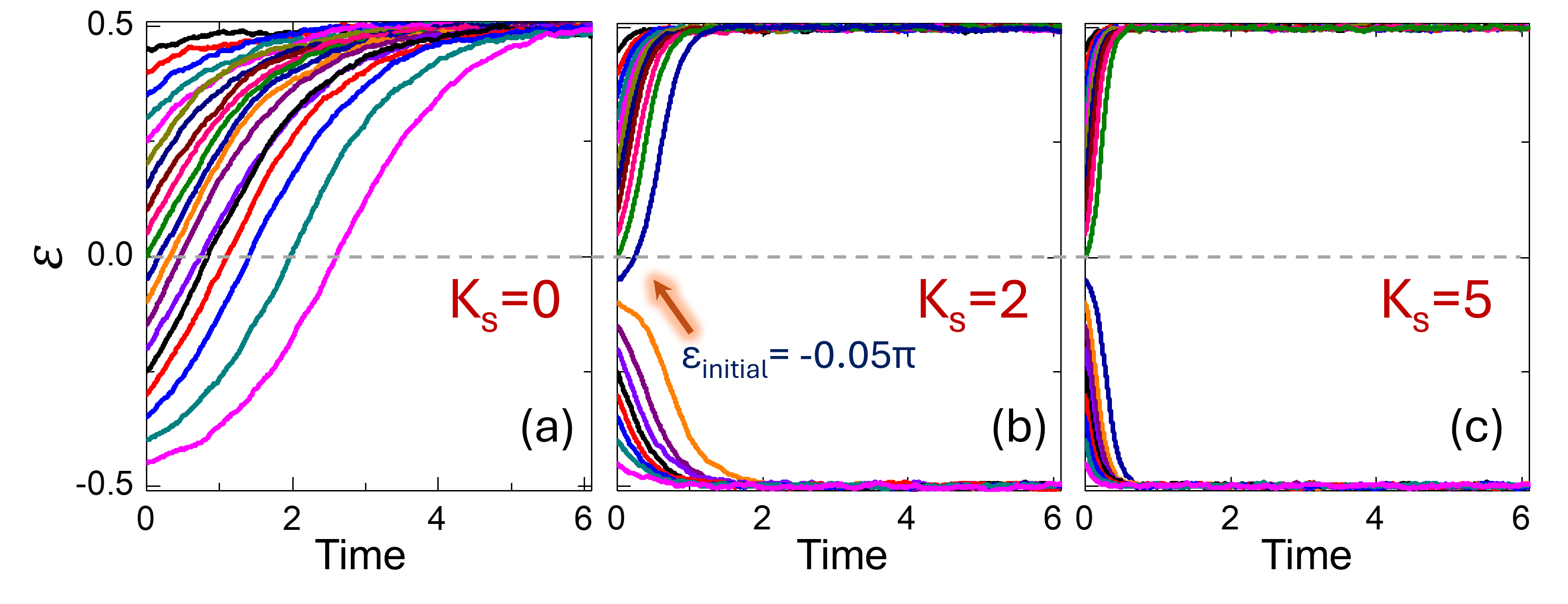
## Line Chart: Oscillation Damping vs. Time with Varying Spring Constants ### Overview The image presents three line charts, arranged horizontally, illustrating the damping of oscillations over time. Each chart corresponds to a different spring constant (Ks) value: 0, 2, and 5. The y-axis represents the angular frequency (ω), and the x-axis represents time. Each chart displays multiple lines representing different initial conditions. A label indicates an initial condition of εinitial = -0.05π. ### Components/Axes * **Y-axis Label:** ω (Angular Frequency) - Scale ranges from approximately -0.5 to 0.5. * **X-axis Label:** Time - Scale ranges from 0 to 6. * **Chart (a):** Ks = 0. Displays multiple oscillating lines. * **Chart (b):** Ks = 2. Displays multiple lines that quickly dampen to around 0. * **Chart (c):** Ks = 5. Displays lines that almost immediately settle at 0. * **Annotation:** εinitial = -0.05π, with an arrow pointing to a line in chart (a). * **Sub-labels:** (a), (b), (c) denoting the different spring constant values. ### Detailed Analysis or Content Details **Chart (a) - Ks = 0:** * **Trend:** Multiple lines exhibit sustained oscillations with varying amplitudes and frequencies. * **Data Points (approximate):** * Black Line: Starts at ~0.45, oscillates around 0, with a period of ~1.5. * Red Line: Starts at ~0.45, oscillates around 0, with a period of ~1.5. * Green Line: Starts at ~-0.45, oscillates around 0, with a period of ~1.5. * Blue Line: Starts at ~-0.45, oscillates around 0, with a period of ~1.5. * Purple Line: Starts at ~0.45, oscillates around 0, with a period of ~1.5. * Cyan Line: Starts at ~-0.45, oscillates around 0, with a period of ~1.5. * The line indicated by the annotation (εinitial = -0.05π) is a cyan line, starting at approximately -0.45. **Chart (b) - Ks = 2:** * **Trend:** Lines quickly dampen towards ω = 0, with some initial oscillations. The damping is significantly faster than in chart (a). * **Data Points (approximate):** * Black Line: Starts at ~0.45, quickly decays to 0 within ~2 time units. * Red Line: Starts at ~0.45, quickly decays to 0 within ~2 time units. * Green Line: Starts at ~-0.45, quickly decays to 0 within ~2 time units. * Blue Line: Starts at ~-0.45, quickly decays to 0 within ~2 time units. * Purple Line: Starts at ~0.45, quickly decays to 0 within ~2 time units. * Cyan Line: Starts at ~-0.45, quickly decays to 0 within ~2 time units. **Chart (c) - Ks = 5:** * **Trend:** Lines almost immediately settle at ω = 0, indicating very rapid damping. * **Data Points (approximate):** * Black Line: Starts at ~0.45, almost immediately decays to 0. * Red Line: Starts at ~0.45, almost immediately decays to 0. * Green Line: Starts at ~-0.45, almost immediately decays to 0. * Blue Line: Starts at ~-0.45, almost immediately decays to 0. * Purple Line: Starts at ~0.45, almost immediately decays to 0. * Cyan Line: Starts at ~-0.45, almost immediately decays to 0. ### Key Observations * Increasing the spring constant (Ks) dramatically reduces the oscillation period and increases the damping rate. * When Ks = 0, the system exhibits sustained oscillations. * As Ks increases, the oscillations are quickly suppressed, and the system returns to equilibrium (ω = 0). * The initial condition (εinitial = -0.05π) does not appear to significantly affect the overall damping trend, only the initial direction of the oscillation. ### Interpretation The charts demonstrate the effect of spring constant (Ks) on the damping of oscillations. A higher spring constant introduces a stronger restoring force, which dissipates energy more rapidly, leading to faster damping. The system transitions from undamped oscillations (Ks = 0) to critically damped or overdamped behavior (Ks = 5). The initial condition influences the starting point of the oscillation but doesn't alter the fundamental damping behavior dictated by the spring constant. This suggests a model of a damped harmonic oscillator where the spring constant plays a crucial role in controlling the system's stability and response to disturbances. The consistent behavior across different initial conditions indicates the system's robustness to small variations in starting state.

## Line Graphs: Time Evolution of ε for Different \( K_s \) Values ### Overview The image contains three horizontally arranged line graphs (subplots (a), (b), (c)) showing the time evolution of the variable \( \boldsymbol{\varepsilon} \) (epsilon) over **Time** (0 to 6) for three values of \( K_s \) (0, 2, 5). Each graph has multiple colored lines (representing different initial conditions/parameters) and shared axes: - **Y-axis**: \( \varepsilon \) (range: \( -0.5 \) to \( 0.5 \)). - **X-axis**: Time (range: \( 0 \) to \( 6 \)). ### Components/Axes - **Y-axis**: Label “\( \varepsilon \)” (epsilon), scale from \( -0.5 \) (bottom) to \( 0.5 \) (top). - **X-axis**: Label “Time”, scale from \( 0 \) (left) to \( 6 \) (right). - **Subplots**: - (a): \( K_s = 0 \) (label in red, bottom-right of subplot). - (b): \( K_s = 2 \) (label in red, bottom-right), with additional text “\( \varepsilon_{\text{initial}} = -0.05\pi \)” (blue, middle) and an orange arrow pointing to a line. - (c): \( K_s = 5 \) (label in red, bottom-right). - **Lines**: Multiple colored lines (red, blue, green, orange, purple, etc.) in each subplot (no legend provided; colors represent different initial conditions/parameters). ### Detailed Analysis #### Subplot (a): \( K_s = 0 \) - **Trend**: All lines (regardless of initial \( \varepsilon \)) trend **upward** over Time, converging toward \( \varepsilon = 0.5 \) (top of the y-axis) as Time increases. - **Initial Conditions**: Lines start at various \( \varepsilon \) values (some above 0, some below) but all move toward \( \varepsilon = 0.5 \). No split in behavior; all lines converge to the upper limit. #### Subplot (b): \( K_s = 2 \) - **Trend**: Lines split into two groups: - Lines with **initial \( \varepsilon < 0 \)** (negative) trend **downward** toward \( \varepsilon = -0.5 \) (bottom of the y-axis). - Lines with **initial \( \varepsilon > 0 \)** (positive) trend **upward** toward \( \varepsilon = 0.5 \) (top). - **Annotation**: “\( \varepsilon_{\text{initial}} = -0.05\pi \)” (blue text) with an orange arrow points to a line in the negative \( \varepsilon \) group (trending downward). - **Convergence**: Slower than (c) but faster than (a) for the split groups. #### Subplot (c): \( K_s = 5 \) - **Trend**: Same split as (b) but **faster convergence**: - Lines with initial \( \varepsilon < 0 \) quickly drop to \( \varepsilon = -0.5 \). - Lines with initial \( \varepsilon > 0 \) quickly rise to \( \varepsilon = 0.5 \). - **Convergence Speed**: Faster than (b); lines reach their respective limits (\( \pm 0.5 \)) more rapidly. ### Key Observations - **Effect of \( K_s \)**: As \( K_s \) increases (0 → 2 → 5), the behavior of \( \varepsilon \) over time changes: - \( K_s = 0 \): All lines converge to \( \varepsilon = 0.5 \) (no split). - \( K_s = 2 \): Split behavior (negative initial \( \varepsilon \to -0.5 \), positive \( \to 0.5 \)). - \( K_s = 5 \): Faster split and convergence to \( \pm 0.5 \). - **Initial Condition Impact**: In (b) and (c), the sign of initial \( \varepsilon \) (positive/negative) determines the final \( \varepsilon \) (0.5 or -0.5); in (a), all initial conditions lead to \( \varepsilon = 0.5 \). - **Convergence Speed**: Higher \( K_s \) (5) causes faster convergence to the limits (\( \pm 0.5 \)) than lower \( K_s \) (2), and (a) has no split (all go to 0.5). ### Interpretation The graphs demonstrate how \( K_s \) controls the time evolution of \( \varepsilon \): - For \( K_s = 0 \), the system has **one attractor** (\( \varepsilon = 0.5 \)): all initial \( \varepsilon \) values converge to this single limit. - For \( K_s \geq 2 \), the system has **two attractors** (\( \varepsilon = 0.5 \) for positive initial \( \varepsilon \), \( \varepsilon = -0.5 \) for negative initial \( \varepsilon \)). Higher \( K_s \) (5) accelerates convergence to these attractors. The annotation in (b) highlights a specific initial condition (\( \varepsilon_{\text{initial}} = -0.05\pi \)) to illustrate the negative initial \( \varepsilon \) behavior. This suggests \( K_s \) modulates the number of attractors (1 for \( K_s = 0 \), 2 for \( K_s \geq 2 \)) and the speed of convergence to them.

## Line Graphs: ξ vs Time for Different K_s Values ### Overview Three panels (a, b, c) display the evolution of ξ over time (0–6) for distinct stiffness constants (K_s = 0, 2, 5). Each panel shows multiple colored lines representing different initial conditions or parameters, converging toward ξ = 0 (dashed gray line). ### Components/Axes - **X-axis**: Time (0–6), labeled "Time" in black. - **Y-axis**: ξ (ranging from -0.5 to 0.5), labeled "ξ" in black. - **Legend**: Located on the right side of each panel, mapping colors to K_s values (e.g., red = K_s=0, blue = K_s=2, etc.). - **Dashed Line**: Horizontal line at ξ = 0 across all panels. - **Annotations**: - Panel (b): "ε_initial = -0.05π" (blue arrow pointing to orange line). - Panel (a): "K_s=0" (red text). - Panel (b): "K_s=2" (red text). - Panel (c): "K_s=5" (red text). ### Detailed Analysis #### Panel (a): K_s=0 - **Lines**: 10+ colored lines (red, blue, green, purple, etc.) curve upward, approaching ξ=0 asymptotically. - **Trends**: All lines increase monotonically but never cross ξ=0. - **Key Data**: - Red line (bottom): Starts at ξ ≈ -0.5, reaches ξ ≈ -0.1 by t=6. - Blue line: Starts at ξ ≈ -0.4, reaches ξ ≈ -0.05 by t=6. - Green line: Starts at ξ ≈ -0.3, reaches ξ ≈ 0 by t=6. #### Panel (b): K_s=2 - **Lines**: 10+ colored lines start at ε_initial = -0.05π (≈ -0.157) and rise toward ξ=0. - **Trends**: Lines flatten faster than in (a), with sharper initial slopes. - **Key Data**: - Orange line (highlighted): Starts at ξ ≈ -0.157, reaches ξ ≈ -0.02 by t=2, then plateaus. - Blue line: Starts at ξ ≈ -0.157, reaches ξ ≈ 0 by t=4. - Green line: Starts at ξ ≈ -0.157, overshoots ξ=0 slightly before stabilizing. #### Panel (c): K_s=5 - **Lines**: 10+ colored lines remain nearly flat near ξ=0. - **Trends**: Minimal deviation from ξ=0 across all time. - **Key Data**: - All lines cluster tightly around ξ=0 (within ±0.01). - No significant movement observed. ### Key Observations 1. **Convergence Behavior**: - Higher K_s values (5 > 2 > 0) result in faster convergence to ξ=0. - At K_s=5, the system stabilizes immediately; at K_s=0, convergence is slowest. 2. **Initial Condition Impact**: - Panel (b) shows a deliberate perturbation (ε_initial = -0.05π), causing transient oscillations before stabilization. 3. **Color Consistency**: - Legend colors match line colors across panels (e.g., red = K_s=0 in all panels). ### Interpretation The graphs model a damped system approaching equilibrium (ξ=0) with stiffness-dependent dynamics: - **K_s=0**: No damping; system evolves slowly toward equilibrium. - **K_s=2**: Moderate damping; initial perturbations decay with oscillations. - **K_s=5**: Overdamped; system stabilizes instantly without overshoot. The ε_initial perturbation in (b) demonstrates how initial displacements are mitigated by increasing K_s. The dashed ξ=0 line serves as a universal reference for equilibrium across all conditions.