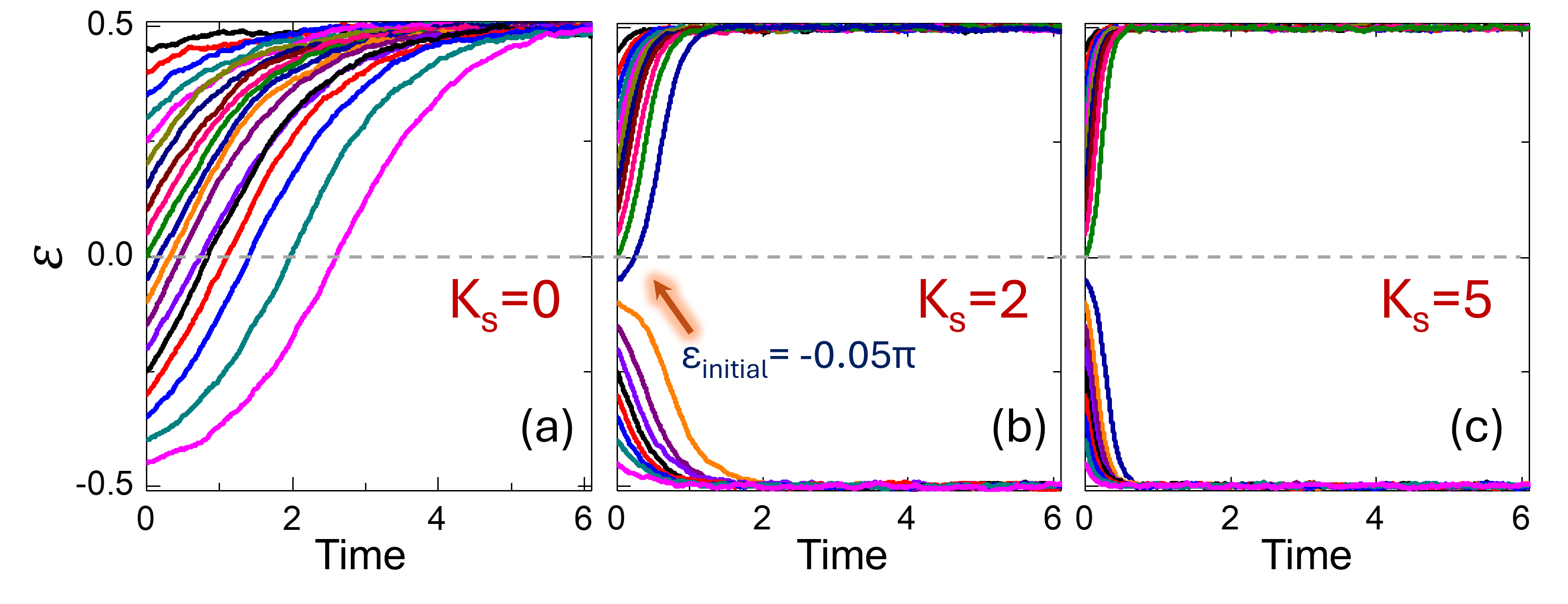
## Line Graphs: Time Evolution of ε for Different \( K_s \) Values ### Overview The image contains three horizontally arranged line graphs (subplots (a), (b), (c)) showing the time evolution of the variable \( \boldsymbol{\varepsilon} \) (epsilon) over **Time** (0 to 6) for three values of \( K_s \) (0, 2, 5). Each graph has multiple colored lines (representing different initial conditions/parameters) and shared axes: - **Y-axis**: \( \varepsilon \) (range: \( -0.5 \) to \( 0.5 \)). - **X-axis**: Time (range: \( 0 \) to \( 6 \)). ### Components/Axes - **Y-axis**: Label “\( \varepsilon \)” (epsilon), scale from \( -0.5 \) (bottom) to \( 0.5 \) (top). - **X-axis**: Label “Time”, scale from \( 0 \) (left) to \( 6 \) (right). - **Subplots**: - (a): \( K_s = 0 \) (label in red, bottom-right of subplot). - (b): \( K_s = 2 \) (label in red, bottom-right), with additional text “\( \varepsilon_{\text{initial}} = -0.05\pi \)” (blue, middle) and an orange arrow pointing to a line. - (c): \( K_s = 5 \) (label in red, bottom-right). - **Lines**: Multiple colored lines (red, blue, green, orange, purple, etc.) in each subplot (no legend provided; colors represent different initial conditions/parameters). ### Detailed Analysis #### Subplot (a): \( K_s = 0 \) - **Trend**: All lines (regardless of initial \( \varepsilon \)) trend **upward** over Time, converging toward \( \varepsilon = 0.5 \) (top of the y-axis) as Time increases. - **Initial Conditions**: Lines start at various \( \varepsilon \) values (some above 0, some below) but all move toward \( \varepsilon = 0.5 \). No split in behavior; all lines converge to the upper limit. #### Subplot (b): \( K_s = 2 \) - **Trend**: Lines split into two groups: - Lines with **initial \( \varepsilon < 0 \)** (negative) trend **downward** toward \( \varepsilon = -0.5 \) (bottom of the y-axis). - Lines with **initial \( \varepsilon > 0 \)** (positive) trend **upward** toward \( \varepsilon = 0.5 \) (top). - **Annotation**: “\( \varepsilon_{\text{initial}} = -0.05\pi \)” (blue text) with an orange arrow points to a line in the negative \( \varepsilon \) group (trending downward). - **Convergence**: Slower than (c) but faster than (a) for the split groups. #### Subplot (c): \( K_s = 5 \) - **Trend**: Same split as (b) but **faster convergence**: - Lines with initial \( \varepsilon < 0 \) quickly drop to \( \varepsilon = -0.5 \). - Lines with initial \( \varepsilon > 0 \) quickly rise to \( \varepsilon = 0.5 \). - **Convergence Speed**: Faster than (b); lines reach their respective limits (\( \pm 0.5 \)) more rapidly. ### Key Observations - **Effect of \( K_s \)**: As \( K_s \) increases (0 → 2 → 5), the behavior of \( \varepsilon \) over time changes: - \( K_s = 0 \): All lines converge to \( \varepsilon = 0.5 \) (no split). - \( K_s = 2 \): Split behavior (negative initial \( \varepsilon \to -0.5 \), positive \( \to 0.5 \)). - \( K_s = 5 \): Faster split and convergence to \( \pm 0.5 \). - **Initial Condition Impact**: In (b) and (c), the sign of initial \( \varepsilon \) (positive/negative) determines the final \( \varepsilon \) (0.5 or -0.5); in (a), all initial conditions lead to \( \varepsilon = 0.5 \). - **Convergence Speed**: Higher \( K_s \) (5) causes faster convergence to the limits (\( \pm 0.5 \)) than lower \( K_s \) (2), and (a) has no split (all go to 0.5). ### Interpretation The graphs demonstrate how \( K_s \) controls the time evolution of \( \varepsilon \): - For \( K_s = 0 \), the system has **one attractor** (\( \varepsilon = 0.5 \)): all initial \( \varepsilon \) values converge to this single limit. - For \( K_s \geq 2 \), the system has **two attractors** (\( \varepsilon = 0.5 \) for positive initial \( \varepsilon \), \( \varepsilon = -0.5 \) for negative initial \( \varepsilon \)). Higher \( K_s \) (5) accelerates convergence to these attractors. The annotation in (b) highlights a specific initial condition (\( \varepsilon_{\text{initial}} = -0.05\pi \)) to illustrate the negative initial \( \varepsilon \) behavior. This suggests \( K_s \) modulates the number of attractors (1 for \( K_s = 0 \), 2 for \( K_s \geq 2 \)) and the speed of convergence to them.