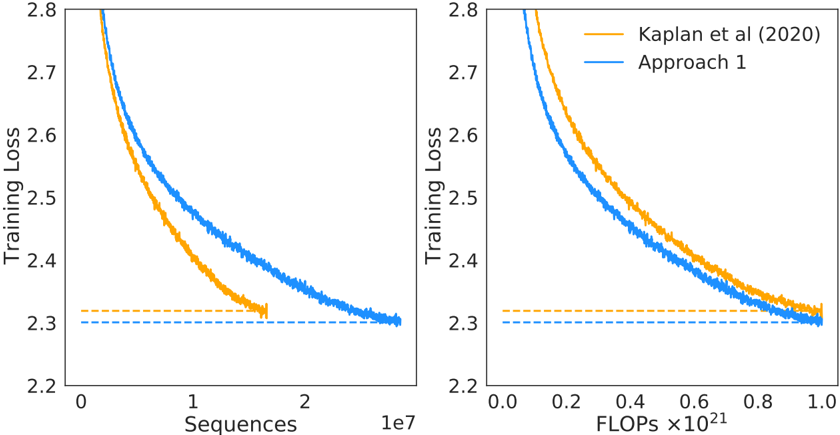
## Line Graph: Training Loss vs. Sequences and FLOPs ### Overview The image contains two line graphs comparing the training loss of two approaches: "Kaplan et al. (2020)" (orange line) and "Approach 1" (blue line). The left graph plots training loss against the number of sequences (0 to 2×10⁷), while the right graph plots training loss against FLOPs (0 to 1×10²¹). Both graphs include a horizontal dashed line at a training loss of 2.3, likely representing a target or baseline value. --- ### Components/Axes - **Left Graph (Sequences)**: - **X-axis**: "Sequences" (logarithmic scale, 0 to 2×10⁷). - **Y-axis**: "Training Loss" (linear scale, 2.2 to 2.8). - **Legend**: Located in the top-right corner, with orange for "Kaplan et al. (2020)" and blue for "Approach 1". - **Dashed Line**: Horizontal line at y=2.3 (both graphs). - **Right Graph (FLOPs)**: - **X-axis**: "FLOPs ×10²¹" (linear scale, 0 to 1×10²¹). - **Y-axis**: "Training Loss" (linear scale, 2.2 to 2.8). - **Legend**: Same as the left graph (orange and blue). - **Dashed Line**: Horizontal line at y=2.3. --- ### Detailed Analysis #### Left Graph (Sequences) - **Kaplan et al. (2020)** (orange): - Starts at ~2.8 training loss at 0 sequences. - Decreases sharply to ~2.3 by ~1×10⁷ sequences. - Fluctuates slightly but stabilizes near 2.3. - **Approach 1** (blue): - Starts at ~2.7 training loss at 0 sequences. - Decreases gradually to ~2.3 by ~2×10⁷ sequences. - Shows minor oscillations but converges to 2.3. #### Right Graph (FLOPs) - **Kaplan et al. (2020)** (orange): - Starts at ~2.8 training loss at 0 FLOPs. - Decreases steeply to ~2.3 by ~0.8×10²¹ FLOPs. - Stabilizes near 2.3. - **Approach 1** (blue): - Starts at ~2.7 training loss at 0 FLOPs. - Decreases gradually to ~2.3 by ~1.0×10²¹ FLOPs. - Converges to 2.3 with minor fluctuations. --- ### Key Observations 1. **Convergence**: Both approaches converge to the same training loss (~2.3), but Kaplan et al. (2020) achieves this faster in both sequence and FLOP metrics. 2. **Efficiency**: Kaplan et al. (2020) demonstrates a steeper decline in training loss, suggesting higher efficiency per sequence or FLOP. 3. **Dashed Line**: The horizontal line at 2.3 likely represents a target or theoretical minimum training loss. 4. **Scalability**: The right graph (FLOPs) shows that Kaplan et al. (2020) requires fewer computational resources (FLOPs) to reach the target loss compared to Approach 1. --- ### Interpretation The data suggests that **Kaplan et al. (2020)** is more computationally efficient than Approach 1, achieving the same training loss with fewer sequences or FLOPs. The convergence to 2.3 indicates that both methods are effective, but Kaplan et al. (2020) outperforms in terms of resource utilization. The dashed line at 2.3 may represent a benchmark or optimization goal, highlighting the importance of balancing training loss and computational cost in model development. The steeper decline in Kaplan et al. (2020) could imply architectural or algorithmic improvements that reduce redundancy or improve gradient propagation.