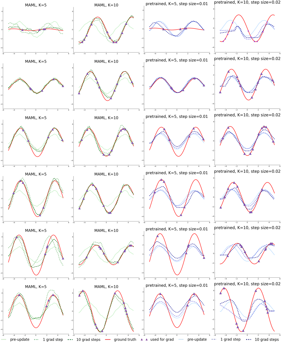
## [Chart Type]: Grid of Regression Plots Comparing Meta-Learning (MAML) and Pretrained Models ### Overview The image displays a 6x4 grid of 24 individual regression plots. Each plot shows the performance of a machine learning model in fitting a sinusoidal function, given a small number of data points (K=5 or K=10). The grid compares two model types: "MAML" (Model-Agnostic Meta-Learning) and "pretrained" models, across different numbers of gradient update steps. The plots visualize how the model's prediction evolves from an initial state ("pre-update") after 1 and 10 gradient steps, relative to the true function ("ground truth"). ### Components/Axes * **Grid Structure:** 6 rows by 4 columns. * **Column Titles (Top of each column):** * Column 1: `MAML, K=5` * Column 2: `MAML, K=10` * Column 3: `pretrained, K=5, step size=0.01` * Column 4: `pretrained, K=10, step size=0.02` * **Axes (All plots share the same scale):** * X-axis: Range approximately -6 to 6. No explicit axis title. * Y-axis: Range approximately -4 to 4. No explicit axis title. * **Legend (Bottom center of the entire figure):** * **For MAML plots (Columns 1 & 2):** * `pre-update`: Light green, dotted line. * `1 grad step`: Medium green, dotted line. * `10 grad steps`: Dark green, dotted line. * `ground truth`: Red, solid line. * `used for grad`: Purple, upward-pointing triangle markers. * **For Pretrained plots (Columns 3 & 4):** * `pre-update`: Light blue, dotted line. * `1 grad step`: Medium blue, dotted line. * `10 grad steps`: Dark blue, dotted line. * `ground truth`: Red, solid line. * `used for grad`: Purple, upward-pointing triangle markers. ### Detailed Analysis **General Pattern per Plot:** 1. A red solid line (`ground truth`) represents a target sine wave with varying amplitude and phase across rows. 2. Purple triangles (`used for grad`) mark the K=5 or K=10 data points sampled from the ground truth, used to train the model for that specific task. 3. A dotted line shows the model's prediction function at three stages: * **Pre-update:** The model's initial guess before seeing the task-specific data points. * **After 1 gradient step:** The model's first adaptation. * **After 10 gradient steps:** The model's more refined adaptation. **Column-wise Trends:** * **Column 1 (MAML, K=5):** The `pre-update` (light green) line is often a poor fit. After 1 gradient step (medium green), the fit improves noticeably, aligning closer to the red line and purple triangles. After 10 steps (dark green), the fit is generally very close to the ground truth, capturing the sine wave's shape well. * **Column 2 (MAML, K=10):** Similar pattern to Column 1, but with more data points (K=10). The adaptation from `pre-update` to `1 grad step` is often more dramatic, and the `10 grad steps` line frequently achieves an excellent fit, sometimes nearly indistinguishable from the ground truth. * **Column 3 (Pretrained, K=5, step size=0.01):** The `pre-update` (light blue) line is often a reasonable, smooth approximation. The updates after 1 and 10 gradient steps (medium and dark blue) show incremental refinement. The final fit (`10 grad steps`) is good but may show slight phase shifts or amplitude mismatches compared to the MAML results. * **Column 4 (Pretrained, K=10, step size=0.02):** With more data and a larger step size, the adaptation is more aggressive. The `pre-update` line is adjusted more significantly after 1 step, and the `10 grad steps` line often fits the data points very closely, though it may occasionally overshoot or exhibit less smoothness than the MAML fits. **Row-wise Variation:** The rows appear to represent different random sinusoidal tasks (different amplitudes and phases). The relative performance trends between columns remain consistent across these different tasks. ### Key Observations 1. **Adaptation Speed:** MAML models (green lines) show a more dramatic and accurate adaptation from the `pre-update` state after just 1 gradient step compared to the pretrained models (blue lines). 2. **Final Fit Quality:** With 10 gradient steps, both MAML and pretrained models achieve good fits. However, the MAML fits (dark green) often appear to match the ground truth (red) more precisely in shape and phase, especially in the K=10 cases. 3. **Effect of K:** Increasing K from 5 to 10 improves the final fit quality for both model types, as expected with more data. 4. **Effect of Step Size:** The pretrained model in Column 4 uses a larger step size (0.02 vs. 0.01), leading to more pronounced changes per step, which can be beneficial but also risks instability. 5. **Pre-update Baseline:** The MAML `pre-update` model is often a very poor, flat guess, while the pretrained `pre-update` model starts as a smoother, more reasonable average function. This highlights MAML's meta-learning objective: to find an initialization that is highly sensitive and adaptable, not necessarily accurate on average. ### Interpretation This figure demonstrates the core advantage of meta-learning (MAML) over standard pretraining for few-shot learning scenarios. The data suggests: * **MAML learns to learn quickly:** The MAML model's initialization (`pre-update`) is not a good fit for any specific task, but it is optimized to require only a few gradient steps to specialize effectively. This is evidenced by the large, accurate jumps from light green to medium/dark green lines. * **Pretrained models adapt more gradually:** The pretrained model starts with a better average representation (`pre-update` blue line) but adapts more slowly and incrementally (smaller changes between blue lines). Its adaptation is more dependent on hyperparameters like step size. * **Efficiency in data-scarce regimes:** For tasks with very few samples (K=5 or 10), MAML's ability to rapidly specialize from a poorly fitting but highly adaptable starting point leads to more accurate final models. The plots show MAML often converging to a closer match of the ground truth function's shape. * **Underlying Principle:** The figure visually validates the meta-learning hypothesis: an initialization trained across many tasks for rapid adaptation will outperform a model simply pretrained on a large dataset when faced with new, data-scarce tasks. The "ground truth" red line represents the new task, and the green lines show the swift, effective specialization of the meta-learned model.