# Technical Document Extraction: Prediction Algorithm Performance
## 1. Document Metadata
* **Title:** Prediction Algorithm Performance
* **Image Type:** 2D Scatter Plot with Classification Boundary
* **Primary Language:** English
* **Coordinate System:** Cartesian ($x_0, x_1$)
## 2. Component Isolation
### A. Header
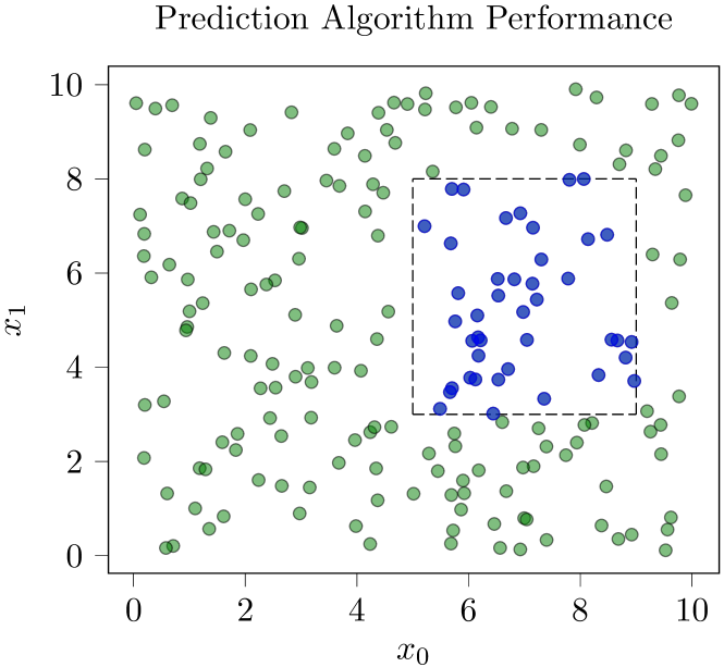
* **Text:** "Prediction Algorithm Performance"
* **Placement:** Centered at the top of the image.
### B. Main Chart Area (Axes and Data)
* **X-Axis Label ($x_0$):** Located at the bottom center.
* **X-Axis Scale:** Numerical markers at 0, 2, 4, 6, 8, and 10.
* **Y-Axis Label ($x_1$):** Located at the left center, rotated 90 degrees.
* **Y-Axis Scale:** Numerical markers at 0, 2, 4, 6, 8, and 10.
* **Background:** Light gray grid-less field.
### C. Data Series and Classification
The plot contains approximately 150-170 individual data points categorized by color and spatial location.
* **Series 1: Green Circles (Negative/Background Class)**
* **Visual Trend:** These points are distributed across the entire $10 \times 10$ plane, except for a specific rectangular region in the mid-right quadrant.
* **Spatial Distribution:** High density in the ranges $x_0 \in [0, 5]$ and $x_0 \in [9, 10]$, and $x_1 \in [0, 3]$ and $x_1 \in [8, 10]$.
* **Outliers/Anomalies:** There is one green point located inside the dashed boundary at approximately $[x_0 \approx 7, x_1 \approx 0.8]$ and another near $[x_0 \approx 3, x_1 \approx 7]$.
* **Series 2: Blue Circles (Positive/Target Class)**
* **Visual Trend:** These points are clustered tightly within a specific rectangular region.
* **Spatial Distribution:** Concentrated within the bounds of $x_0 \in [5, 9]$ and $x_1 \in [3, 8]$.
### D. Decision Boundary (Dashed Box)
* **Type:** Rectangular dashed line.
* **Coordinates:**
* **Bottom-Left Corner:** $[5.0, 3.0]$
* **Top-Right Corner:** $[9.0, 8.0]$
* **Function:** This represents the algorithm's prediction zone. Points inside the box are predicted as the "Blue" class; points outside are predicted as the "Green" class.
## 3. Data Analysis and Observations
### Classification Accuracy
* **True Positives (Blue points inside the box):** The majority of blue points (approx. 45-50 points) are correctly contained within the dashed boundary.
* **False Positives (Green points inside the box):** There are no green points visible inside the dashed boundary, suggesting high precision for the "Blue" class.
* **False Negatives (Blue points outside the box):** There are no blue points visible outside the dashed boundary, suggesting high recall for the "Blue" class.
* **True Negatives (Green points outside the box):** The vast majority of green points are correctly located outside the dashed boundary.
### Summary of Spatial Logic
The algorithm has defined a rectangular decision rule:
$IF (5.0 \leq x_0 \leq 9.0) \text{ AND } (3.0 \leq x_1 \leq 8.0) \text{ THEN Class = Blue, ELSE Class = Green.}$
Based on the visual evidence, this algorithm achieves near-perfect separation of the two classes in this specific feature space.