## Composite Image: Causal Diagrams and Ternary Plots ### Overview The image presents four sub-figures, labeled (a) through (d). Sub-figures (a) and (c) are causal diagrams showing relationships between variables, while (b) and (d) are ternary plots representing probability distributions. ### Components/Axes **Sub-figure (a): Causal Diagram** * Nodes: A, B * Edges: * λ (lambda) -> A (downward arrow) * ν (nu) -> B (downward arrow) * A -> B (rightward arrow) **Sub-figure (b): Ternary Plot** * Vertices: [00], [01], [10], [11] * Plot Type: Ternary plot with a flat, evenly distributed surface. **Sub-figure (c): Causal Diagram** * Nodes: A, B * Edges: * λ (lambda) -> A (downward arrow) * ν (nu) -> B (downward arrow) **Sub-figure (d): Ternary Plot** * Vertices: [00], [01], [10], [11] * Plot Type: Ternary plot with a curved surface, concentrated near the [01] vertex. ### Detailed Analysis **Sub-figure (a): Causal Diagram** * Variable λ influences A. * Variable ν influences B. * A influences B. **Sub-figure (b): Ternary Plot** * The plot shows a uniform distribution across the ternary space defined by the vertices [00], [01], [10], and [11]. The color gradient appears smooth and consistent across the entire surface. **Sub-figure (c): Causal Diagram** * Variable λ influences A. * Variable ν influences B. **Sub-figure (d): Ternary Plot** * The plot shows a non-uniform distribution, with the highest values concentrated near the [01] vertex. The surface curves significantly, indicating a strong bias towards the [01] state. ### Key Observations * Sub-figures (a) and (c) depict different causal relationships. (a) includes a direct influence of A on B, while (c) only shows influences on A and B from λ and ν, respectively. * Sub-figures (b) and (d) represent different probability distributions on a ternary space. (b) shows a uniform distribution, while (d) shows a distribution heavily skewed towards the [01] vertex. ### Interpretation The image likely illustrates the impact of different causal structures on the resulting probability distributions. The causal diagram in (a) with the direct influence of A on B results in a uniform distribution in (b). In contrast, the causal diagram in (c) without the direct influence of A on B results in a skewed distribution in (d), concentrated at [01]. This suggests that the causal relationships between variables significantly affect the probability distributions over the possible states. The variables λ and ν likely represent some underlying factors that influence A and B, and the absence of a direct link between A and B in (c) leads to a specific distribution pattern in (d).

\n ## Diagram: Quantum State Transitions and Bloch Sphere Representations ### Overview The image presents four diagrams illustrating concepts related to quantum mechanics, specifically focusing on state transitions and their representation on the Bloch sphere. Diagrams (a) and (c) depict state transitions between two levels, labeled A and B, influenced by external factors represented by λ and ν. Diagrams (b) and (d) show 3D representations resembling Bloch spheres, with coordinate labels indicating specific quantum states. ### Components/Axes * **Diagram (a) & (c):** * Labels: λ, ν, A, B * Arrows: Downward arrows labeled λ and ν, and a horizontal arrow from A to B. * **Diagram (b) & (d):** * Coordinate Labels: [00], [01], [10], [11] are labeled on the vertices of the triangular shape. * Surface: A 3D surface with color gradients. ### Detailed Analysis or Content Details * **Diagram (a):** Shows a transition from state A to state B. A downward arrow labeled "λ" points towards A, and another downward arrow labeled "ν" points towards B. An arrow connects A to B, indicating a transition. * **Diagram (c):** Similar to (a), shows a transition from state A to state B. A downward arrow labeled "λ" points towards A, and another downward arrow labeled "ν" points towards B. An arrow connects A to B, indicating a transition. * **Diagram (b):** Displays a triangular surface with coordinate labels at the vertices: [00], [01], [10], and [11]. The surface exhibits a color gradient, transitioning from red to blue. The shape resembles a Bloch sphere representation. * **Diagram (d):** Similar to (b), displays a triangular surface with coordinate labels at the vertices: [00], [01], [10], and [11]. The surface exhibits a color gradient, transitioning from red to blue. The shape resembles a Bloch sphere representation. ### Key Observations * Diagrams (a) and (c) are structurally identical, suggesting they represent the same physical process or scenario. * Diagrams (b) and (d) are also structurally identical, representing the same Bloch sphere configuration. * The coordinate labels [00], [01], [10], and [11] likely represent the basis states of a two-qubit system. * The color gradients in (b) and (d) likely represent the probability amplitude or some other quantum property associated with each state. ### Interpretation The diagrams likely illustrate the effect of external influences (λ and ν) on the transition between two quantum states (A and B). Diagrams (b) and (d) provide a visual representation of the resulting quantum state on the Bloch sphere. The coordinate labels indicate the basis states, and the color gradients represent the probability amplitudes or other quantum properties. The similarity between (a) and (c), and (b) and (d) suggests that the diagrams are presenting different perspectives of the same underlying quantum phenomenon. The diagrams could be used to explain concepts such as quantum state manipulation, decoherence, or entanglement. The diagrams do not provide specific numerical data, but rather a qualitative representation of quantum processes. The absence of numerical values limits the extent to which detailed quantitative analysis can be performed. However, the diagrams are valuable for visualizing and understanding the fundamental principles of quantum mechanics.

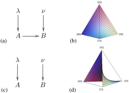
## Diagram and Plot Composite: Directed Graphs and 3D Surface Visualizations ### Overview The image is a composite figure containing four distinct sub-figures, labeled (a), (b), (c), and (d). It appears to be from a technical or scientific document, likely illustrating concepts in causal modeling, probability, or information theory. The left column shows directed acyclic graphs (DAGs), and the right column shows corresponding 3D surface plots over a binary domain. ### Components/Axes The image is divided into a 2x2 grid. * **Top-Left (a):** A directed graph with four nodes labeled with Greek and Latin letters. Arrows indicate directed relationships. * **Top-Right (b):** A 3D surface plot. The base is a square with vertices labeled with binary pairs: `[00]` (bottom-left), `[01]` (top), `[10]` (right), and `[11]` (bottom-right). A colored surface is plotted above this base. * **Bottom-Left (c):** A directed graph similar to (a), but with a different connection structure. * **Bottom-Right (d):** A 3D surface plot similar to (b), but with a different surface shape. It shares the same axis labels: `[00]`, `[01]`, `[10]`, `[11]`. **Textual Elements Extracted:** * **Sub-figure Labels:** `(a)`, `(b)`, `(c)`, `(d)` are placed below each respective panel. * **Graph Node Labels (a & c):** `λ` (lambda), `ν` (nu), `A`, `B`. * **Plot Axis Labels (b & d):** `[00]`, `[01]`, `[10]`, `[11]`. These are positioned at the four corners of the base plane of the 3D plots. ### Detailed Analysis **Panel (a): Directed Graph** * **Components:** Four nodes. * **Flow/Relationships:** 1. Node `λ` has a directed edge pointing to node `A`. 2. Node `ν` has a directed edge pointing to node `B`. 3. Node `A` has a directed edge pointing to node `B`. * **Interpretation:** This structure suggests `A` is influenced by `λ`, and `B` is influenced by both `ν` and `A`. `A` mediates the influence of `λ` on `B`. **Panel (b): 3D Surface Plot** * **Axes:** The base plane is defined by two binary variables, creating four discrete points: (0,0), (0,1), (1,0), (1,1), labeled as `[00]`, `[01]`, `[10]`, `[11]`. * **Surface:** A smooth, continuous surface is plotted over this domain. The surface is highest at the `[01]` vertex and slopes downward towards the other vertices, with the lowest point appearing near `[10]`. The surface is colored with a gradient (blue/purple to red/yellow), likely representing the Z-axis value (height). * **Trend:** The surface shows a clear peak at the coordinate corresponding to `[01]`. **Panel (c): Directed Graph** * **Components:** Same four nodes as in (a): `λ`, `ν`, `A`, `B`. * **Flow/Relationships:** 1. Node `λ` has a directed edge pointing to node `A`. 2. Node `ν` has a directed edge pointing to node `B`. 3. **Crucially, there is NO edge from `A` to `B`.** * **Interpretation:** This structure suggests `A` and `B` are independent, each influenced only by their respective parent nodes (`λ` and `ν`). There is no causal link or direct dependency between `A` and `B`. **Panel (d): 3D Surface Plot** * **Axes:** Identical to panel (b): `[00]`, `[01]`, `[10]`, `[11]`. * **Surface:** A different smooth surface is plotted. This surface is highest at the `[01]` vertex and slopes down sharply towards the `[11]` vertex, creating a pronounced curved "valley" along the edge from `[01]` to `[11]`. The surface is relatively flat and low along the edge from `[00]` to `[10]`. The color gradient is similar to (b). * **Trend:** The surface shows a peak at `[01]` and a significant, non-linear dip towards `[11]`. ### Key Observations 1. **Structural Contrast:** The primary contrast is between the connected graph in (a) and the disconnected graph in (c). The edge `A → B` is present in (a) but absent in (c). 2. **Surface Contrast:** The surface in (b) appears more symmetric and bowl-like, while the surface in (d) is highly asymmetric with a sharp curvature along one diagonal. 3. **Label Consistency:** The axis labels `[00]`, `[01]`, `[10]`, `[11]` are consistent between plots (b) and (d), allowing for direct comparison of the surfaces. 4. **Color Mapping:** The color gradient on the surfaces (blue/purple for lower values, transitioning to red/yellow for higher values) is consistent, aiding in visual comparison of relative heights. ### Interpretation This figure likely illustrates the relationship between causal structure and the shape of a joint probability distribution or a related function (like a utility or payoff function). * **Graph (a) to Plot (b):** The connected graph where `A` influences `B` may correspond to a distribution where the variables `A` and `B` are dependent. The surface in (b) could represent the joint probability `P(A, B)` or a function `f(A, B)`. The smooth, single-peaked shape suggests a specific type of dependency. * **Graph (c) to Plot (d):** The disconnected graph, implying `A` and `B` are independent, corresponds to a different surface shape in (d). The sharp curvature and distinct valley suggest a more complex or constrained relationship, possibly illustrating a scenario where independence leads to a different functional form, or perhaps showing the effect of removing the `A → B` link on the resulting distribution. **Underlying Message:** The figure demonstrates that a change in the underlying causal or dependency structure (removing the arrow from `A` to `B`) leads to a qualitatively different outcome in the associated mathematical object visualized by the surface plot. It visually argues that structure dictates function. The specific meaning of `λ`, `ν`, the surfaces, and the binary labels would be defined in the accompanying text of the source document, but the visual comparison is clear.

## Diagram and 3D Plot Analysis: Material Transformation and Stress Distribution ### Overview The image contains two distinct sections: 1. **Diagrams (a) and (c)**: Arrows labeled with variables (λ, ν) and states (A, B) suggesting directional relationships or transformations. 2. **3D Plots (b) and (d)**: Tetrahedral structures with color gradients and labeled axes ([00], [10], [11], [01]), likely representing crystallographic orientations or stress/strain distributions. --- ### Components/Axes #### Diagrams (a) and (c): - **Labels**: - **A** and **B**: States or phases (e.g., initial/final configurations). - **λ** and **ν**: Parameters (e.g., wavelength, Poisson’s ratio, or transformation coefficients). - **Flow**: - Diagram (a): A → B with λ and ν acting as directional forces. - Diagram (c): A ← B with λ and ν reversed, implying a feedback or iterative process. #### 3D Plots (b) and (d): - **Axes**: - **X-axis**: [00] (reference plane). - **Y-axis**: [10] (primary crystallographic direction). - **Z-axis**: [11] and [01] (secondary crystallographic directions). - **Color Gradient**: - **Blue to Red**: Likely represents magnitude (e.g., stress intensity, strain energy). - **White Regions**: Absence of data or neutral zones. --- ### Detailed Analysis #### Diagrams (a) and (c): - **Diagram (a)**: - λ and ν act as **input forces** driving the transformation from A to B. - Spatial grounding: λ is positioned above A, ν above B, suggesting sequential application. - **Diagram (c)**: - λ and ν now act as **output forces** from B to A, indicating a reverse process or equilibrium state. - Spatial grounding: λ and ν are positioned below A and B, respectively, emphasizing feedback. #### 3D Plots (b) and (d): - **Plot (b)**: - Color gradient transitions from **blue ([00])** to **red ([01])**, peaking at [11]. - Suggests highest intensity (e.g., stress) at [11] orientation. - **Plot (d)**: - Color gradient shifts to **purple ([00])** and **yellow ([10])**, with a white void at [11]. - Indicates reduced intensity or material failure at [11] under altered conditions. --- ### Key Observations 1. **Reversal of Forces**: Diagram (c) inverts the direction of λ and ν compared to (a), implying a dynamic system (e.g., cyclic loading). 2. **Stress Concentration**: 3D Plot (b) highlights [11] as a critical zone, while Plot (d) shows material degradation at this orientation. 3. **Color Correlation**: Blue (low intensity) and red (high intensity) align with typical stress visualization conventions. --- ### Interpretation - **Material Behavior**: The diagrams likely model phase transformations (A → B) under mechanical parameters (λ, ν), while the 3D plots visualize resultant stress/strain distributions. - **Critical Failure**: The white void in Plot (d) at [11] suggests a fracture or phase boundary under specific conditions. - **Dynamic Equilibrium**: The bidirectional arrows in (a) and (c) may represent hysteresis or reversible transformations in the material. --- **Note**: No explicit numerical data or legends are present in the image. Trends and interpretations are based on standard conventions for stress/strain visualization and crystallographic analysis.