## Composite Image: Causal Diagrams and Ternary Plots
### Overview
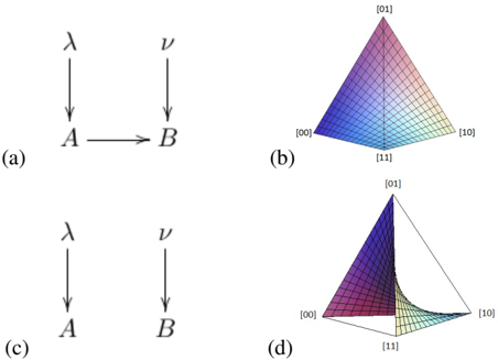
The image presents four sub-figures, labeled (a) through (d). Sub-figures (a) and (c) are causal diagrams showing relationships between variables, while (b) and (d) are ternary plots representing probability distributions.
### Components/Axes
**Sub-figure (a): Causal Diagram**
* Nodes: A, B
* Edges:
* λ (lambda) -> A (downward arrow)
* ν (nu) -> B (downward arrow)
* A -> B (rightward arrow)
**Sub-figure (b): Ternary Plot**
* Vertices: [00], [01], [10], [11]
* Plot Type: Ternary plot with a flat, evenly distributed surface.
**Sub-figure (c): Causal Diagram**
* Nodes: A, B
* Edges:
* λ (lambda) -> A (downward arrow)
* ν (nu) -> B (downward arrow)
**Sub-figure (d): Ternary Plot**
* Vertices: [00], [01], [10], [11]
* Plot Type: Ternary plot with a curved surface, concentrated near the [01] vertex.
### Detailed Analysis
**Sub-figure (a): Causal Diagram**
* Variable λ influences A.
* Variable ν influences B.
* A influences B.
**Sub-figure (b): Ternary Plot**
* The plot shows a uniform distribution across the ternary space defined by the vertices [00], [01], [10], and [11]. The color gradient appears smooth and consistent across the entire surface.
**Sub-figure (c): Causal Diagram**
* Variable λ influences A.
* Variable ν influences B.
**Sub-figure (d): Ternary Plot**
* The plot shows a non-uniform distribution, with the highest values concentrated near the [01] vertex. The surface curves significantly, indicating a strong bias towards the [01] state.
### Key Observations
* Sub-figures (a) and (c) depict different causal relationships. (a) includes a direct influence of A on B, while (c) only shows influences on A and B from λ and ν, respectively.
* Sub-figures (b) and (d) represent different probability distributions on a ternary space. (b) shows a uniform distribution, while (d) shows a distribution heavily skewed towards the [01] vertex.
### Interpretation
The image likely illustrates the impact of different causal structures on the resulting probability distributions. The causal diagram in (a) with the direct influence of A on B results in a uniform distribution in (b). In contrast, the causal diagram in (c) without the direct influence of A on B results in a skewed distribution in (d), concentrated at [01]. This suggests that the causal relationships between variables significantly affect the probability distributions over the possible states. The variables λ and ν likely represent some underlying factors that influence A and B, and the absence of a direct link between A and B in (c) leads to a specific distribution pattern in (d).