## Diagram: Iterative Causal Discovery Process Using a Large Language Model (LLM)
### Overview
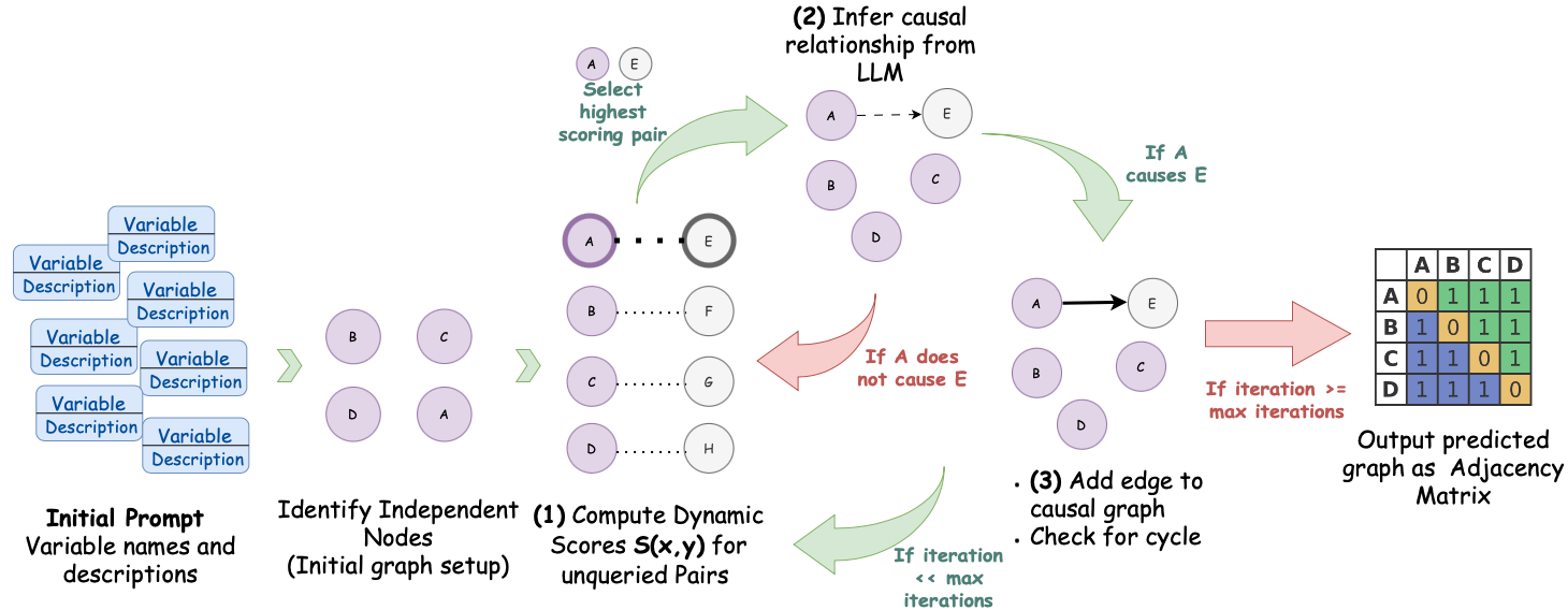
The image is a flowchart illustrating a multi-step, iterative process for constructing a causal graph from a set of variable descriptions. The process uses a Large Language Model (LLM) to infer causal relationships between pairs of variables, dynamically scores potential pairs, and builds an adjacency matrix as the final output. The flow is cyclical, with decisions based on the LLM's inference and iteration counts.
### Components/Axes
The diagram is organized into a left-to-right flow with a feedback loop. Key components are:
1. **Initial Prompt (Far Left):** A stack of blue boxes labeled "Variable Description".
2. **Identify Independent Nodes (Left-Center):** Four purple circles labeled B, C, D, A, representing the initial graph setup.
3. **(1) Compute Dynamic Scores S(x,y) for unqueried Pairs (Center):** A vertical list of variable pairs (A-E, B-F, C-G, D-H) with dotted lines, indicating potential relationships to be scored.
4. **(2) Infer causal relationship from LLM (Top-Center):** A cluster of nodes (A, B, C, D, E) with a dashed arrow from A to E, representing the LLM's hypothesis.
5. **Decision Point (Center-Right):** Two large, curved arrows:
* A **green arrow** labeled "If A causes E" points to the next step.
* A **red arrow** labeled "If A does not cause E" points back to the scoring step.
6. **(3) Add edge to causal graph / Check for cycle (Right-Center):** The graph now shows a solid black arrow from A to E.
7. **Iteration Check (Right):** A large red arrow labeled "If iteration >= max iterations" points to the final output.
8. **Output (Far Right):** A 4x4 grid labeled "Output predicted graph as Adjacency Matrix" with rows and columns for A, B, C, D.
### Detailed Analysis
**Process Flow:**
1. **Initialization:** The process begins with an "Initial Prompt" containing variable names and descriptions. This leads to the identification of independent nodes (A, B, C, D), forming the initial graph.
2. **Scoring & Selection:** The system computes dynamic scores `S(x,y)` for unqueried pairs of variables (e.g., A-E, B-F). The pair with the highest score (A-E) is selected for investigation.
3. **LLM Inference:** The selected pair (A, E) is presented to an LLM to infer a causal relationship. The diagram shows a hypothesized dashed arrow from A to E.
4. **Decision & Action:**
* **If the LLM infers A causes E (Green Path):** A solid edge is added from A to E in the causal graph, and the system checks for cycles.
* **If the LLM infers A does NOT cause E (Red Path):** The process loops back to the scoring step to evaluate the next highest-scoring pair.
5. **Iteration & Termination:** The cycle of scoring, inferring, and adding edges continues. The process terminates when the iteration count reaches a predefined maximum (`max iterations`), at which point the final causal graph is output as an adjacency matrix.
**Adjacency Matrix Content:**
The final output is a 4x4 matrix with rows and columns labeled A, B, C, D. The values are:
```
A B C D
A 0 1 1 1
B 1 0 1 1
C 1 1 0 1
D 1 1 1 0
```
This matrix indicates a fully connected graph where every variable has a directed edge to every other variable (e.g., A→B, A→C, A→D, B→A, etc.), except for self-loops (the diagonal is all 0s).
### Key Observations
1. **Iterative and Dynamic:** The process is not a one-shot inference. It dynamically selects which variable pair to query next based on computed scores, making it adaptive.
2. **LLM as Oracle:** The core causal judgment is delegated to an LLM, which acts as a knowledge oracle for each queried pair.
3. **Cycle Checking:** A critical step after adding an edge is to check for cycles, ensuring the resulting graph remains a valid Directed Acyclic Graph (DAG), which is fundamental for causal models.
4. **Termination Condition:** The process is bounded by a maximum number of iterations, preventing infinite loops and providing a stopping rule.
5. **Final Graph Density:** The example adjacency matrix shows a complete graph (every node connected to every other node). This may be a simplified example for illustration, as real-world causal graphs are typically sparser.
### Interpretation
This diagram outlines a **human-in-the-loop-style algorithmic framework** where an LLM automates the discovery of causal structures. The "Peircean investigative" reading suggests this is an abductive process: the system observes data (variable descriptions), generates hypotheses about causal links (via the LLM), and iteratively tests and refines the model.
The significance lies in automating a task that traditionally requires deep domain expertise. By breaking the problem into pairwise queries and using dynamic scoring, the method attempts to efficiently navigate the vast space of possible causal relationships. The final adjacency matrix is a machine-readable representation of the discovered causal knowledge, ready for use in further analysis, such as causal inference or simulation. The presence of a max iteration count acknowledges the computational and practical limits of exhaustive discovery. The example's fully connected output matrix likely serves to clearly demonstrate the format, rather than represent a realistic outcome, which would typically show a more nuanced and sparse structure reflecting true causal dependencies.