## 2D Parametric Plot: Phase Portrait of a Dynamical System
### Overview
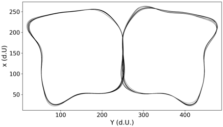
The image displays a 2D line plot featuring two symmetric, closed-loop curves plotted on a Cartesian coordinate system. The visual pattern resembles a butterfly or a figure-eight, characteristic of phase space representations in dynamical systems. The plot consists of multiple overlapping black lines, suggesting either a system with slight noise, multiple iterations of a periodic orbit, or a strange attractor.
### Components/Axes
* **Vertical Axis (Y-axis):** Labeled "x (d.U.)".
* Scale: Ranges from 50 to 250.
* Ticks: Marked at 50, 100, 150, 200, 250.
* **Horizontal Axis (X-axis):** Labeled "Y (d.U.)".
* Scale: Ranges from 100 to 400 (with visual data extending beyond these bounds).
* Ticks: Marked at 100, 200, 300, 400.
* **Data Series:**
* The data is represented by thin, black, continuous lines.
* The lines are not singular; they appear as a bundle of overlapping traces, indicating a high degree of consistency across multiple cycles or data points.
* **Units:** The label "(d.U.)" likely stands for "dimensionless units" or "data units."
### Detailed Analysis
* **Left Loop:**
* **Spatial Position:** Occupies the left side of the chart, centered roughly around Y ≈ 150.
* **Trend:** The curve starts near the center (Y ≈ 250, X ≈ 125), sweeps outward to the left (reaching a minimum Y value of approximately 50), curves upward to a maximum X value of approximately 255, and returns to the center.
* **Right Loop:**
* **Spatial Position:** Occupies the right side of the chart, centered roughly around Y ≈ 350.
* **Trend:** The curve mirrors the left loop, sweeping outward to the right (reaching a maximum Y value of approximately 470), curving upward to a maximum X value of approximately 260, and returns to the center.
* **Intersection/Convergence:**
* Both loops converge at a central point located approximately at Y ≈ 250 and X ≈ 125. This appears to be a critical point or a saddle point in the phase space.
* **Bounds:**
* The system is bounded vertically between X ≈ 25 and X ≈ 265.
* The system is bounded horizontally between Y ≈ 30 and Y ≈ 470.
### Key Observations
* **Symmetry:** The plot exhibits strong bilateral symmetry across the vertical axis line Y = 250.
* **Line Thickness/Jitter:** The lines are not perfectly sharp, indicating that the system is either slightly noisy or that the trajectory is not perfectly periodic (i.e., it does not trace the exact same path every time, but stays within a tight "tube" of probability).
* **Curvature:** The curves are smooth, indicating a continuous dynamical system rather than a discrete map.
### Interpretation
* **Nature of the Data:** This is a classic phase portrait. The "butterfly" shape is highly reminiscent of the Lorenz attractor or similar coupled oscillator systems.
* **System Behavior:** The convergence at the center (Y ≈ 250, X ≈ 125) suggests a point of instability or a saddle point through which the system trajectory passes repeatedly. The two loops represent the "wings" of the attractor, where the system oscillates between two distinct states or regions of phase space.
* **Stability:** The fact that the lines are tightly bundled suggests that the system is in a stable limit cycle or a well-defined strange attractor. The slight "fuzziness" or thickness of the lines indicates that the system is not perfectly deterministic or is subject to minor perturbations, yet it remains confined to a specific region of the phase space.
* **Peircean Investigative Note:** The visual evidence suggests a system that is deterministic but complex. The symmetry implies that the underlying differential equations governing this system likely contain symmetric terms (e.g., a potential well with two minima). The "d.U." units suggest this is a simulation or a normalized experimental result rather than raw sensor data.