## Scatter Plot Grid: Correlation Functions vs. Momentum Difference
### Overview
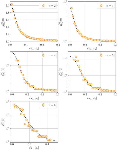
The image presents a grid of five scatter plots. Each plot displays the correlation function g^(n)_k⊥(0) as a function of the momentum difference δk⊥[kd] for different values of 'n' (n=2, 3, 4, 5, and 6). The y-axis is linear for n=2 and logarithmic for n=3, 4, 5, and 6. Each data point is represented by an orange circle with error bars. A dashed black line is overlaid on each plot, representing a theoretical fit to the data.
### Components/Axes
* **Arrangement:** The plots are arranged in a 2x3 grid, with the bottom-right position empty.
* **X-axis:**
* Label: δk⊥[kd]
* Scale: Linear, ranging from 0.0 to approximately 0.3 for n=2, and from 0.0 to approximately 0.6 for n=3, 4, 5, and 6.
* **Y-axis:**
* Label: g^(n)_k⊥(0)
* Scale:
* n=2: Linear, ranging from 1.0 to 2.0.
* n=3, 4, 5, 6: Logarithmic (base 10).
* n=3: Ranges from 10^0 (1) to 10^1 (10).
* n=4: Ranges from 10^0 (1) to 10^2 (100).
* n=5: Ranges from 10^0 (1) to 10^2 (100).
* n=6: Ranges from 10^0 (1) to 10^3 (1000).
* **Data Points:** Orange circles with error bars.
* **Fit Line:** Dashed black line representing a theoretical fit.
* **Titles:** Each plot has a title indicating the value of 'n': n=2 (top-left), n=3 (top-right), n=4 (middle-left), n=5 (middle-right), n=6 (bottom-left).
### Detailed Analysis
**Plot for n=2:**
* Trend: The correlation function decreases rapidly as δk⊥[kd] increases.
* Data Points:
* At δk⊥[kd] = 0.0, g^(2)_k⊥(0) ≈ 2.0.
* At δk⊥[kd] = 0.1, g^(2)_k⊥(0) ≈ 1.2.
* At δk⊥[kd] = 0.2, g^(2)_k⊥(0) ≈ 1.05.
* At δk⊥[kd] = 0.3, g^(2)_k⊥(0) ≈ 1.0.
**Plot for n=3:**
* Trend: The correlation function decreases rapidly as δk⊥[kd] increases.
* Data Points:
* At δk⊥[kd] = 0.0, g^(3)_k⊥(0) ≈ 8.0.
* At δk⊥[kd] = 0.1, g^(3)_k⊥(0) ≈ 1.5.
* At δk⊥[kd] = 0.2, g^(3)_k⊥(0) ≈ 0.8.
* At δk⊥[kd] = 0.6, g^(3)_k⊥(0) ≈ 0.3.
**Plot for n=4:**
* Trend: The correlation function decreases rapidly as δk⊥[kd] increases, then plateaus.
* Data Points:
* At δk⊥[kd] = 0.0, g^(4)_k⊥(0) ≈ 150.
* At δk⊥[kd] = 0.1, g^(4)_k⊥(0) ≈ 10.
* At δk⊥[kd] = 0.2, g^(4)_k⊥(0) ≈ 2.
* For δk⊥[kd] > 0.3, g^(4)_k⊥(0) ≈ 1.
**Plot for n=5:**
* Trend: The correlation function decreases rapidly as δk⊥[kd] increases, then plateaus.
* Data Points:
* At δk⊥[kd] = 0.0, g^(5)_k⊥(0) ≈ 120.
* At δk⊥[kd] = 0.1, g^(5)_k⊥(0) ≈ 8.
* At δk⊥[kd] = 0.2, g^(5)_k⊥(0) ≈ 2.
* For δk⊥[kd] > 0.3, g^(5)_k⊥(0) ≈ 1.
**Plot for n=6:**
* Trend: The correlation function decreases rapidly as δk⊥[kd] increases, then plateaus.
* Data Points:
* At δk⊥[kd] = 0.0, g^(6)_k⊥(0) ≈ 600.
* At δk⊥[kd] = 0.1, g^(6)_k⊥(0) ≈ 30.
* At δk⊥[kd] = 0.2, g^(6)_k⊥(0) ≈ 5.
* For δk⊥[kd] > 0.4, g^(6)_k⊥(0) ≈ 1.
### Key Observations
* As 'n' increases, the initial value of the correlation function g^(n)_k⊥(0) at δk⊥[kd] = 0.0 increases significantly.
* For n=4, 5, and 6, the correlation function plateaus at a value close to 1 for larger values of δk⊥[kd].
* The theoretical fit (dashed black line) appears to match the data reasonably well in all plots.
### Interpretation
The plots illustrate how the correlation function g^(n)_k⊥(0) changes with the momentum difference δk⊥[kd] for different values of 'n'. The rapid decrease in the correlation function at small δk⊥[kd] suggests a strong correlation at short distances, which diminishes as the distance increases. The plateau observed for n=4, 5, and 6 indicates that the correlation function approaches a constant value at larger momentum differences. The increasing initial value of the correlation function with increasing 'n' suggests that the correlation strength is dependent on the parameter 'n'. The theoretical fit provides a model for the relationship between the correlation function and the momentum difference, which can be used to further analyze the underlying physical processes.