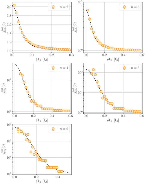
## Multi-Panel Scatter/Line Plot: Correlation Functions $g_{\delta k_\perp}^{(n)}(0)$ ### Overview The image displays a grid of five sub-plots illustrating the behavior of a correlation function, denoted as $g_{\delta k_\perp}^{(n)}(0)$, plotted against the variable $\delta k_\perp$ (in units of $k_d$). The plots are arranged in a 3-row layout (two plots in the top row, two in the middle, and one in the bottom). Each plot corresponds to a specific integer value of $n$, ranging from $n=2$ to $n=6$. The data is presented as orange circles with vertical error bars, overlaid with a dashed black line representing a theoretical fit. ### Components/Axes * **Common Axes:** * **X-axis:** Labeled $\delta k_\perp [k_d]$ across all plots. The range varies slightly by plot, generally spanning from 0.0 to 0.6. * **Y-axis:** Labeled $g_{\delta k_\perp}^{(n)}(0)$ across all plots. * **Legends:** Each plot contains a legend in the top-right corner identifying the specific $n$ value for that panel ($n=2, 3, 4, 5, 6$). * **Visual Elements:** * **Orange Circles:** Represent experimental or calculated data points. * **Vertical Lines (on circles):** Represent error bars/uncertainty. * **Dashed Black Line:** Represents the theoretical model or trend line. * **Grid:** All plots feature a light gray grid background. --- ### Detailed Analysis #### 1. Top-Left Plot ($n=2$) * **Y-axis Scale:** Linear, ranging from 1.0 to 2.0. * **X-axis Scale:** 0.0 to 0.3. * **Trend:** The data shows a monotonic, smooth decay. It starts at a maximum of approximately 2.05 at $\delta k_\perp = 0$ and decays rapidly, flattening out as it approaches 1.0 near $\delta k_\perp \approx 0.15$. * **Fit:** The dashed line tracks the data points closely throughout the range. #### 2. Top-Right Plot ($n=3$) * **Y-axis Scale:** Logarithmic, ranging from 1 to 10. * **X-axis Scale:** 0.0 to 0.6. * **Trend:** The data exhibits an exponential-like decay. It starts at approximately 6.0 at $\delta k_\perp = 0$ and drops to 1.0 by $\delta k_\perp \approx 0.4$. * **Fit:** The dashed line provides a good fit, though the data points show slight scatter around the line. #### 3. Middle-Left Plot ($n=4$) * **Y-axis Scale:** Logarithmic, ranging from 1 to 100. * **X-axis Scale:** 0.0 to 0.6. * **Trend:** A steep, exponential-like decay. The starting value is approximately 30.0 at $\delta k_\perp = 0$. The value drops significantly, reaching the baseline of 1.0 at $\delta k_\perp \approx 0.4$. * **Fit:** The dashed line follows the trend, but there is noticeable "stair-stepping" or quantization in the data points at the lower end of the Y-axis (near 1.0). #### 4. Middle-Right Plot ($n=5$) * **Y-axis Scale:** Logarithmic, ranging from 1 to 100. * **X-axis Scale:** 0.0 to 0.6. * **Trend:** Similar to $n=4$, but with a higher starting magnitude. The value at $\delta k_\perp = 0$ is approximately 150.0. It decays sharply to 1.0 by $\delta k_\perp \approx 0.4$. * **Fit:** The theoretical line fits the general downward slope, though data points show increased variance compared to lower $n$ values. #### 5. Bottom-Left Plot ($n=6$) * **Y-axis Scale:** Logarithmic, ranging from 1 to 1000. * **X-axis Scale:** 0.0 to 0.5. * **Trend:** The steepest decay of the set. The starting value is approximately 600.0 at $\delta k_\perp = 0$. It decays rapidly, reaching the baseline of 1.0 at $\delta k_\perp \approx 0.4$. * **Fit:** The dashed line captures the overall trend, but the data points exhibit significant scatter, particularly in the range of 10 to 100. --- ### Key Observations * **Magnitude Scaling:** There is a clear positive correlation between the value of $n$ and the initial magnitude of the correlation function at $\delta k_\perp = 0$. As $n$ increases from 2 to 6, the starting value increases from ~2 to ~600. * **Decay Behavior:** In all cases, the correlation function decays as $\delta k_\perp$ increases, eventually saturating at a value of approximately 1.0. * **Saturation Point:** The saturation point (where the function hits ~1.0) appears consistent across the plots, occurring roughly at $\delta k_\perp \approx 0.4$. * **Data Quantization:** In the plots for $n=4, 5, 6$, the data points at the lower end of the Y-axis (near 1.0) appear to align on discrete horizontal levels, suggesting a potential resolution limit or quantization effect in the underlying data generation process. ### Interpretation The data demonstrates the behavior of higher-order correlation functions in a system, likely related to turbulence or statistical field theory. The dramatic increase in the initial value of $g_{\delta k_\perp}^{(n)}(0)$ as $n$ increases indicates that higher-order moments of the distribution are significantly more sensitive to small-scale fluctuations (small $\delta k_\perp$). The convergence to a value of 1.0 at larger $\delta k_\perp$ is characteristic of correlation functions, where the system becomes uncorrelated (or reaches a baseline state) as the separation distance increases. The theoretical dashed lines suggest that the system is well-described by a specific statistical model, though the increased scatter and quantization at higher $n$ values suggest that higher-order moments are more susceptible to noise or require higher sampling density to resolve accurately.