## Line Graphs: Relationship Between δk⊥ and g^(n)_δk⊥(0) for n=2 to 6
### Overview
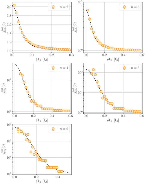
The image contains five line graphs arranged in a 2x2 grid with one additional graph at the bottom right. Each graph represents a different value of the parameter `n` (2–6) and plots the relationship between the perpendicular wavevector deviation `δk⊥` (normalized by `k_d`) and the function `g^(n)_δk⊥(0)` on a logarithmic scale. Data points are represented by orange circles with error bars, and a dashed black reference line is present in all graphs.
---
### Components/Axes
1. **X-Axis**:
- Label: `δk⊥ [k_d]`
- Range: 0.0 to 0.6 (linear scale)
- Position: Bottom of all graphs
2. **Y-Axis**:
- Label: `g^(n)_δk⊥(0)`
- Scales:
- `n=2`: Linear (1.0–2.0)
- `n=3`: Logarithmic (10⁰–10¹)
- `n=4`: Logarithmic (10⁰–10¹)
- `n=5`: Logarithmic (10⁰–10²)
- `n=6`: Logarithmic (10⁰–10³)
- Position: Left of all graphs
3. **Legend**:
- Located in the top-right corner of each graph.
- Format: Orange circle with `n=` value (e.g., `n=2`, `n=3`, etc.).
4. **Data Points**:
- Orange circles with vertical error bars.
- Error bars are small relative to the data points.
5. **Reference Line**:
- Dashed black line in all graphs.
- Position: Overlays data points, suggesting a theoretical or fitted trend.
---
### Detailed Analysis
#### Graph 1: `n=2`
- **Y-Axis Scale**: Linear (1.0–2.0).
- **Trend**: Data points decrease smoothly from ~2.0 at `δk⊥=0.0` to ~1.0 at `δk⊥=0.3`.
- **Error Bars**: Minimal (~±0.05).
#### Graph 2: `n=3`
- **Y-Axis Scale**: Logarithmic (10⁰–10¹).
- **Trend**: Data points drop from ~10¹ at `δk⊥=0.0` to ~10⁰ at `δk⊥=0.6`.
- **Error Bars**: ~±0.1 (log scale).
#### Graph 3: `n=4`
- **Y-Axis Scale**: Logarithmic (10⁰–10¹).
- **Trend**: Similar to `n=3`, but steeper decline.
- **Error Bars**: ~±0.1 (log scale).
#### Graph 4: `n=5`
- **Y-Axis Scale**: Logarithmic (10⁰–10²).
- **Trend**: Data points start at ~10¹ at `δk⊥=0.0` and drop to ~10⁰ at `δk⊥=0.6`.
- **Error Bars**: ~±0.1 (log scale).
#### Graph 5: `n=6`
- **Y-Axis Scale**: Logarithmic (10⁰–10³).
- **Trend**: Sharp initial drop from ~10² at `δk⊥=0.0` to ~10⁰ at `δk⊥=0.4`, then plateaus.
- **Error Bars**: ~±0.1 (log scale).
---
### Key Observations
1. **Universal Decline**: All graphs show a decreasing trend of `g^(n)_δk⊥(0)` with increasing `δk⊥`.
2. **Scale Dependence**: Higher `n` values require logarithmic scales to capture the full range of `g^(n)_δk⊥(0)`.
3. **Convergence**: For `n≥4`, the data points align closely with the dashed reference line, suggesting a consistent theoretical model.
4. **Error Consistency**: Error bars are smallest at `δk⊥=0.0` and grow slightly with increasing `δk⊥`.
---
### Interpretation
The graphs demonstrate that `g^(n)_δk⊥(0)` decreases monotonically with increasing perpendicular wavevector deviation `δk⊥`. The use of logarithmic scales for `n≥3` indicates that the magnitude of `g^(n)_δk⊥(0)` spans several orders of magnitude, particularly for `n=6`. The dashed reference line likely represents a theoretical prediction (e.g., exponential decay or power-law behavior), which the data closely follows. The error bars suggest high precision in measurements, especially at low `δk⊥`.
The parameter `n` may correspond to a system property (e.g., dimensionality, coupling strength, or disorder level). The steeper decline for higher `n` implies that larger `n` values amplify the sensitivity of `g^(n)_δk⊥(0)` to `δk⊥`. This could reflect phenomena such as increased dissipation, localization, or interference effects in a physical system.
The spatial arrangement of graphs emphasizes the systematic variation of `n`, allowing direct comparison of trends across different parameter regimes. The absence of outliers or anomalies suggests robustness in the observed behavior.