## Diagram: Maximum and Projection ### Overview The image presents two 3D surface diagrams, labeled (c) Maximum and (d) Projection. Both diagrams depict surfaces in relation to axes labeled α and β. Diagram (c) shows a surface with a maximum point, while diagram (d) shows a surface with a minimum point. Both diagrams include curves on the surface labeled with κ symbols. ### Components/Axes **Diagram (c) Maximum:** * **Title:** (c) Maximum * **Axes:** * α (horizontal axis) * β (axis extending into the page) * **Surface:** A curved surface with a maximum point. The surface is shaded in varying tones of blue. * **Curves:** Two curves on the surface, intersecting at the maximum point. * Curve 1: Labeled "κ₊^(α,β)" near the maximum point. * Curve 2: Labeled "κ₋^(α,β)" near the maximum point. * **Inequality:** "κ₊^(α,β) < 0, κ₋^(α,β) < 0" is displayed above the surface. **Diagram (d) Projection:** * **Title:** (d) Projection * **Axes:** * α (horizontal axis) * β (axis extending into the page) * **Surface:** A curved surface with a minimum point. The surface is shaded in varying tones of blue. * **Curves:** Two curves on the surface, intersecting at the minimum point. * Curve 1: Labeled "κ₊^(α,β)" near the minimum point. * Curve 2: Labeled "κ₋^(α,β)" near the minimum point. * **Text:** "random directions η, δ" is displayed below the diagram. ### Detailed Analysis **Diagram (c) Maximum:** * The surface appears to be a section of a paraboloid, opening downwards. * The maximum point is located at the intersection of the two curves. * The inequality "κ₊^(α,β) < 0, κ₋^(α,β) < 0" indicates that the curvatures in both directions are negative at the maximum point. **Diagram (d) Projection:** * The surface appears to be a section of a paraboloid, opening upwards. * The minimum point is located at the intersection of the two curves. * The text "random directions η, δ" suggests that the projection is related to random directions. ### Key Observations * Both diagrams depict surfaces with critical points (maximum and minimum). * The curves on the surfaces are labeled with κ symbols, likely representing curvatures. * The inequality in diagram (c) indicates negative curvatures at the maximum point. ### Interpretation The diagrams illustrate the concepts of maximum and projection in relation to a surface defined by parameters α and β. The curvatures (κ₊^(α,β) and κ₋^(α,β)) play a role in characterizing the shape of the surface at these critical points. The negative curvatures at the maximum point in diagram (c) are consistent with the surface being concave downwards. Diagram (d) shows the projection of the surface, potentially along random directions η and δ, resulting in a surface with a minimum point. The relationship between the original surface and its projection is not explicitly defined in the image, but it suggests a transformation or mapping of the surface.

\n ## Diagram: Maximum and Projection Surfaces ### Overview The image presents two 3D diagrams, labeled "(c) Maximum" and "(d) Projection". Both diagrams depict curved surfaces, with labeled axes α and β. The diagram "(c) Maximum" shows a surface with a pronounced peak, and "(d) Projection" shows a surface that extends outwards. Both diagrams feature circular contours and labeled points. ### Components/Axes * **Diagram (c) Maximum:** * Axes: α (horizontal), β (horizontal, angled), Z-axis is implicit (vertical). * Surface: A curved surface resembling a rounded hill or dome. The surface is shaded to indicate depth. * Contours: Two circular contours are present on the peak of the surface. * Labels: * κ⁺^α,β < 0, κ⁻^α,β < 0 (above the peak) * κ⁻^α,β (pointing to the left contour) * κ⁺^α,β (pointing to the right contour) * **Diagram (d) Projection:** * Axes: α (vertical), β (horizontal), Z-axis is implicit (depth). * Surface: A curved surface extending outwards, resembling a hyperbolic paraboloid. The surface is shaded to indicate depth. * Contours: Two circular contours are present. * Labels: * κ⁻^α,β (pointing to the left contour) * κ⁺^α,β (pointing to the right contour) * Text: "random directions η, δ" (bottom-right) ### Detailed Analysis or Content Details * **Diagram (c) Maximum:** * The surface peaks along the β-axis. * The contours indicate lines of constant value on the surface. * The labels κ⁺^α,β and κ⁻^α,β suggest curvature values. The inequality κ⁺^α,β < 0, κ⁻^α,β < 0 indicates that both principal curvatures are negative at the peak, implying a saddle-like point. * **Diagram (d) Projection:** * The surface extends outwards from the origin along the β-axis. * The contours indicate lines of constant value on the surface. * The labels κ⁺^α,β and κ⁻^α,β suggest curvature values. The contours are closer together near the origin, indicating a higher curvature in that region. * The text "random directions η, δ" suggests that the projection is related to random variables or directions. ### Key Observations * Both diagrams use the same labels for the curvature values (κ⁺^α,β and κ⁻^α,β), suggesting a relationship between the two surfaces. * The inequality κ⁺^α,β < 0, κ⁻^α,β < 0 is only present in diagram (c), indicating a specific property of the "Maximum" surface. * The "Projection" surface appears to be a projection of the "Maximum" surface onto a different coordinate system. ### Interpretation These diagrams likely represent mathematical surfaces used in a context involving curvature analysis. The labels κ⁺^α,β and κ⁻^α,β likely denote the principal curvatures of the surface in the α-β plane. The inequality in diagram (c) suggests a specific geometric property of the surface at its peak. The "Projection" diagram may represent a transformation or mapping of the "Maximum" surface, potentially related to random variables or directions as indicated by the text. The diagrams are likely part of a larger mathematical or physical model, possibly related to optimization, signal processing, or statistical mechanics. The diagrams demonstrate the concept of curvature and how it changes across a surface, and how a surface can be projected or transformed.

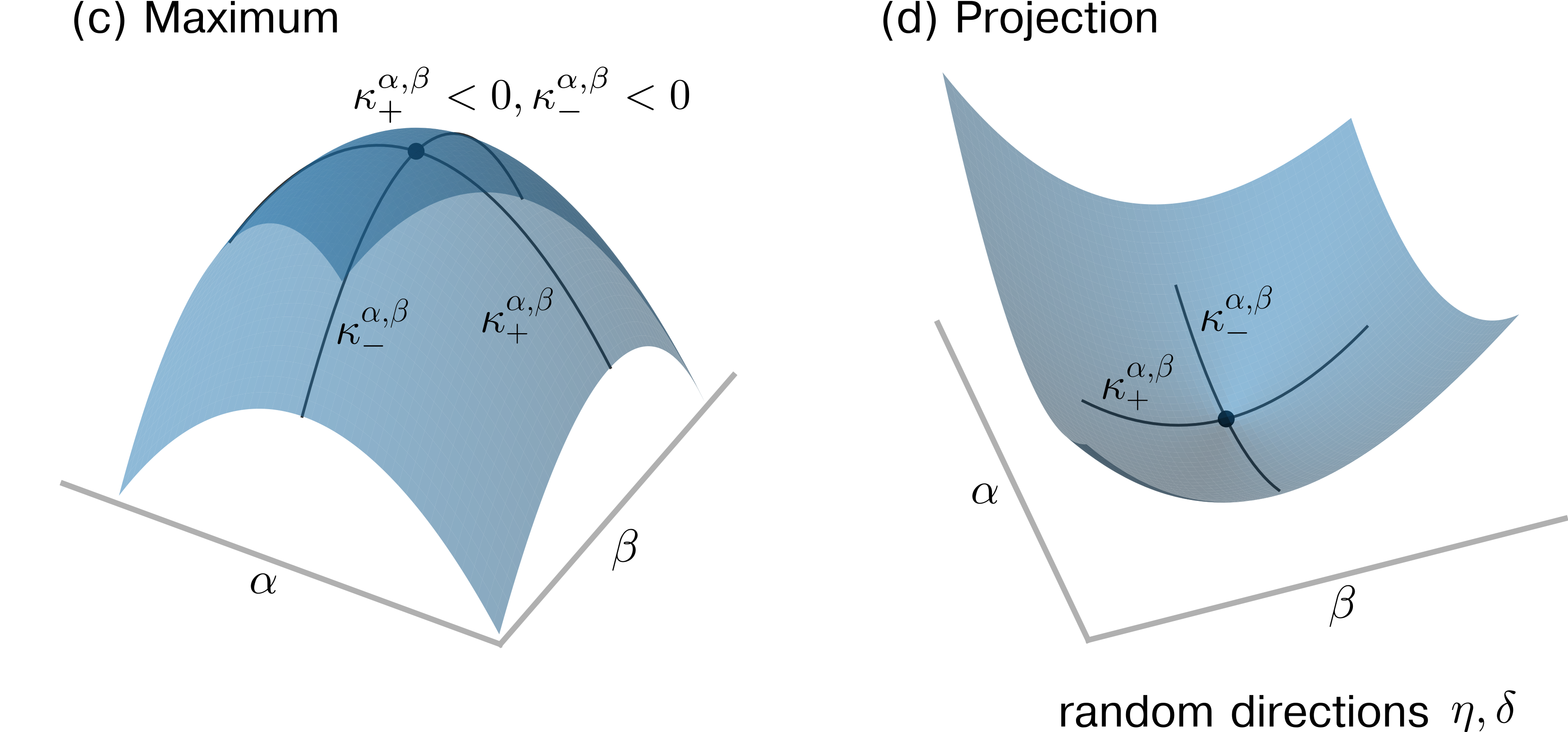
\n ## Mathematical Diagrams: Curvature at Critical Points ### Overview The image displays two 3D surface plots, labeled (c) and (d), illustrating geometric concepts related to curvature at critical points on a surface parameterized by variables α and β. These diagrams are likely from a technical paper on differential geometry, optimization, or manifold learning. ### Components/Axes **Diagram (c) Maximum:** * **Title:** "(c) Maximum" (top-left corner). * **Surface:** A dome-shaped (elliptic paraboloid) surface, concave down. * **Axes:** Two axes labeled with Greek letters: * `α` (alpha) - positioned along the bottom-left edge. * `β` (beta) - positioned along the bottom-right edge. * **Key Point:** A dark dot at the apex (maximum) of the surface. * **Curves:** Two dark curves intersect at the apex, representing principal directions of curvature. * **Labels on Curves:** * `κ₊^{α,β}` (kappa plus, superscript alpha, beta) - labels one curve. * `κ₋^{α,β}` (kappa minus, superscript alpha, beta) - labels the other curve. * **Mathematical Condition:** Text above the apex states: `κ₊^{α,β} < 0, κ₋^{α,β} < 0`. **Diagram (d) Projection:** * **Title:** "(d) Projection" (top-left corner). * **Surface:** A saddle-shaped (hyperbolic paraboloid) surface. * **Axes:** Two axes labeled: * `α` (alpha) - positioned along the left edge. * `β` (beta) - positioned along the bottom edge. * **Key Point:** A dark dot at the saddle point (minimax) of the surface. * **Curves:** Two dark curves intersect at the saddle point. * **Labels on Curves:** * `κ₊^{α,β}` (kappa plus, superscript alpha, beta) - labels one curve. * `κ₋^{α,β}` (kappa minus, superscript alpha, beta) - labels the other curve. * **Additional Text:** Below the diagram, the text "random directions η, δ" is present, where η (eta) and δ (delta) are Greek letters. ### Detailed Analysis **Diagram (c) Maximum:** * **Visual Trend:** The surface curves downward in all directions from the central apex point. * **Component Isolation:** The diagram is segmented into the surface, the intersecting curves, and the axis labels. The mathematical condition is placed directly above the point of interest. * **Spatial Grounding:** The legend/labels (`κ₊^{α,β}`, `κ₋^{α,β}`) are placed directly on their corresponding curves near the apex. The condition `κ₊^{α,β} < 0, κ₋^{α,β} < 0` is positioned at the top-center, directly above the apex dot. * **Data/Fact Extraction:** The diagram explicitly states that at the maximum point, both principal curvatures (`κ₊` and `κ₋`) in the α-β parameterization are negative (`< 0`). This is a defining characteristic of a local maximum on a surface. **Diagram (d) Projection:** * **Visual Trend:** The surface curves upward in one principal direction and downward in the other, creating a saddle shape. * **Component Isolation:** The diagram is segmented into the saddle surface, the intersecting curves, the axis labels, and the standalone text about random directions. * **Spatial Grounding:** The curve labels (`κ₊^{α,β}`, `κ₋^{α,β}`) are placed on their respective curves near the saddle point. The text "random directions η, δ" is placed in the bottom-right corner, separate from the main diagram. * **Data/Fact Extraction:** The diagram shows a saddle point where the principal curvatures have opposite signs (one positive, one negative), though the specific signs are not stated in text. The mention of "random directions η, δ" suggests this projection might relate to analyzing curvature in arbitrary or sampled directions, not just the principal ones. ### Key Observations 1. **Contrasting Geometries:** The two diagrams present a direct visual contrast between a local maximum (all curvatures negative) and a saddle point (curvatures of opposite sign). 2. **Notation Consistency:** The same notation (`κ₊^{α,β}`, `κ₋^{α,β}`) is used for principal curvatures in both diagrams, facilitating comparison. 3. **Contextual Text:** The phrase "random directions η, δ" in diagram (d) is an important annotation that is not present in (c), hinting at a different analytical context for the projection case. ### Interpretation These diagrams serve as visual proofs or illustrations of fundamental concepts in differential geometry applied to optimization or analysis on manifolds. * **What the data suggests:** Diagram (c) demonstrates that for a function or surface to have a local maximum at a point, its Hessian matrix (represented here by the principal curvatures `κ₊` and `κ₋`) must be negative definite. Diagram (d) illustrates a saddle point, where the Hessian is indefinite (has both positive and negative eigenvalues). * **How elements relate:** The axes (α, β) define a local coordinate system on the surface. The curves represent the principal directions of curvature, which are orthogonal at the critical point. The signs of the curvatures along these directions determine the nature of the critical point (max, min, or saddle). * **Notable implications:** The inclusion of "random directions η, δ" in the projection diagram suggests the author may be discussing how curvature behaves when not measured along the principal axes, which is relevant for numerical methods or stochastic analysis where the exact principal directions are unknown. The diagrams collectively emphasize the importance of second-order derivative information (curvature) in classifying critical points.

## 3D Mathematical Diagrams: Maximum and Projection ### Overview The image contains two 3D mathematical diagrams labeled **(c) Maximum** and **(d) Projection**. Both plots use axes labeled **α** and **β**, with surfaces defined by mathematical expressions involving **κ** (kappa) terms with exponents **α, β**. The diagrams appear to represent optimization or stability analysis, with shaded regions and critical points marked. --- ### Components/Axes #### **(c) Maximum** - **Axes**: - Horizontal axes: **α** (x-axis) and **β** (y-axis). - Vertical axis: Implicitly represents the value of the function being maximized. - **Surface**: - A shaded, curved surface with a **peak** (maximum point) at the center. - Labels on the surface: - **κ₊^{α,β} < 0** (top-left edge). - **κ₋^{α,β} < 0** (bottom-right edge). - A critical point is marked at the peak with a dark dot. #### **(d) Projection** - **Axes**: - Horizontal axes: **α** (x-axis) and **β** (y-axis). - Vertical axis: Implicitly represents the projected value. - **Surface**: - A saddle-shaped surface with a **saddle point** marked by a dark dot. - Labels on the surface: - **κ₊^{α,β}** (bottom-left edge). - **κ₋^{α,β}** (top-right edge). - **Additional Text**: - Below both plots: **"random directions η, δ"** (Greek letters eta and delta). --- ### Detailed Analysis #### **(c) Maximum** - The surface is shaded in gradients of blue, with darker regions near the peak. - The inequalities **κ₊^{α,β} < 0** and **κ₋^{α,β} < 0** suggest constraints or conditions for the maximum. - The peak represents the global maximum of the function under the given constraints. #### **(d) Projection** - The saddle shape indicates a critical point where the function transitions from concave to convex. - The labels **κ₊^{α,β}** and **κ₋^{α,β}** likely denote directional derivatives or curvature terms in the projection. - The term **"random directions η, δ"** implies stochastic or multi-directional analysis. --- ### Key Observations 1. **Symmetry**: Both plots share the same axes (**α, β**) but differ in surface geometry (peak vs. saddle). 2. **Critical Points**: - **(c)** has a single maximum point. - **(d)** has a saddle point, suggesting a local extremum with mixed curvature. 3. **Mathematical Context**: The use of **κ** terms with exponents **α, β** hints at a parameterized system, possibly in physics or optimization. --- ### Interpretation - The diagrams likely model a system where **α** and **β** are parameters influencing stability or optimization. - The **maximum** plot (c) could represent a stable equilibrium, while the **projection** (d) might illustrate sensitivity to perturbations (e.g., random directions **η, δ**). - The inequalities **κ₊^{α,β} < 0** and **κ₋^{α,β} < 0** in (c) suggest that the maximum is bounded by negative curvature terms, possibly indicating stability. - The saddle point in (d) implies a bifurcation or transition point in the system’s behavior. No numerical data or legends are present, so trends cannot be quantified. The focus is on symbolic relationships between parameters and curvature terms.