## 3D Mathematical Diagrams: Maximum and Projection
### Overview
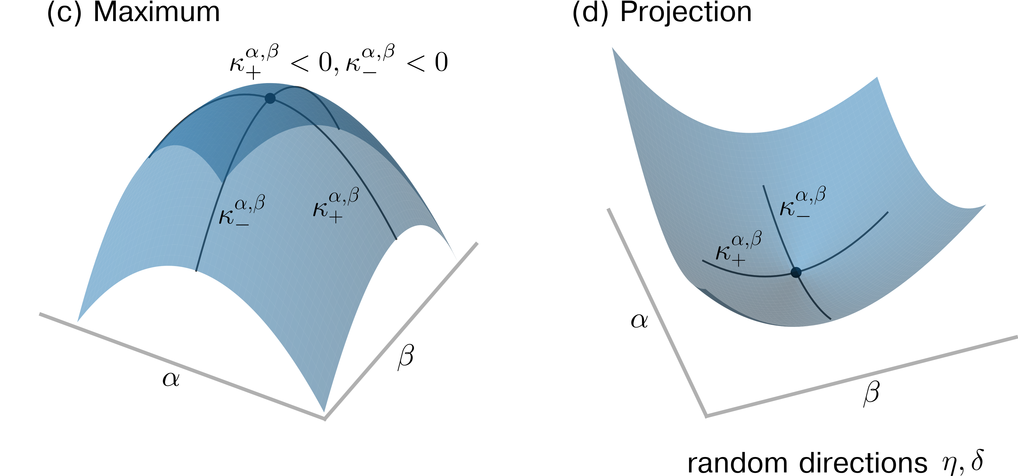
The image contains two 3D mathematical diagrams labeled **(c) Maximum** and **(d) Projection**. Both plots use axes labeled **α** and **β**, with surfaces defined by mathematical expressions involving **κ** (kappa) terms with exponents **α, β**. The diagrams appear to represent optimization or stability analysis, with shaded regions and critical points marked.
---
### Components/Axes
#### **(c) Maximum**
- **Axes**:
- Horizontal axes: **α** (x-axis) and **β** (y-axis).
- Vertical axis: Implicitly represents the value of the function being maximized.
- **Surface**:
- A shaded, curved surface with a **peak** (maximum point) at the center.
- Labels on the surface:
- **κ₊^{α,β} < 0** (top-left edge).
- **κ₋^{α,β} < 0** (bottom-right edge).
- A critical point is marked at the peak with a dark dot.
#### **(d) Projection**
- **Axes**:
- Horizontal axes: **α** (x-axis) and **β** (y-axis).
- Vertical axis: Implicitly represents the projected value.
- **Surface**:
- A saddle-shaped surface with a **saddle point** marked by a dark dot.
- Labels on the surface:
- **κ₊^{α,β}** (bottom-left edge).
- **κ₋^{α,β}** (top-right edge).
- **Additional Text**:
- Below both plots: **"random directions η, δ"** (Greek letters eta and delta).
---
### Detailed Analysis
#### **(c) Maximum**
- The surface is shaded in gradients of blue, with darker regions near the peak.
- The inequalities **κ₊^{α,β} < 0** and **κ₋^{α,β} < 0** suggest constraints or conditions for the maximum.
- The peak represents the global maximum of the function under the given constraints.
#### **(d) Projection**
- The saddle shape indicates a critical point where the function transitions from concave to convex.
- The labels **κ₊^{α,β}** and **κ₋^{α,β}** likely denote directional derivatives or curvature terms in the projection.
- The term **"random directions η, δ"** implies stochastic or multi-directional analysis.
---
### Key Observations
1. **Symmetry**: Both plots share the same axes (**α, β**) but differ in surface geometry (peak vs. saddle).
2. **Critical Points**:
- **(c)** has a single maximum point.
- **(d)** has a saddle point, suggesting a local extremum with mixed curvature.
3. **Mathematical Context**: The use of **κ** terms with exponents **α, β** hints at a parameterized system, possibly in physics or optimization.
---
### Interpretation
- The diagrams likely model a system where **α** and **β** are parameters influencing stability or optimization.
- The **maximum** plot (c) could represent a stable equilibrium, while the **projection** (d) might illustrate sensitivity to perturbations (e.g., random directions **η, δ**).
- The inequalities **κ₊^{α,β} < 0** and **κ₋^{α,β} < 0** in (c) suggest that the maximum is bounded by negative curvature terms, possibly indicating stability.
- The saddle point in (d) implies a bifurcation or transition point in the system’s behavior.
No numerical data or legends are present, so trends cannot be quantified. The focus is on symbolic relationships between parameters and curvature terms.