## Line Graphs: Qwen2.5-7B-Math Attention Weights Across Layers
### Overview
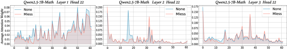
The image contains three line graphs comparing attention weight distributions across three transformer layers (Layer 1, Layer 2, Layer 3) of the Qwen2.5-7B-Math model. Each graph compares two conditions: "None" (blue line) and "Mless" (orange line). The x-axis represents attention weight values (0-60), while the y-axis shows normalized attention magnitudes. The graphs reveal distinct patterns of attention concentration across layers and conditions.
### Components/Axes
- **X-axis**: "Average Attention Weight" (0-60, integer intervals)
- **Y-axis**: Normalized attention magnitude (ranges vary per layer):
- Layer 1: 0.00-0.08
- Layer 2: 0.00-0.200
- Layer 3: 0.00-0.175
- **Legends**:
- Blue line: "None" (no modification)
- Orange line: "Mless" (modified condition)
- **Graph Titles**:
- Layer 1: "Qwen2.5-7B-Math Layer 1 Head 22"
- Layer 2: "Qwen2.5-7B-Math Layer 2 Head 22"
- Layer 3: "Qwen2.5-7B-Math Layer 3 Head 22"
### Detailed Analysis
#### Layer 1
- **None (blue)**: Peaks at x=15 (0.065), x=35 (0.072), and x=55 (0.068). Baseline values cluster between 0.01-0.03.
- **Mless (orange)**: Peaks at x=10 (0.055), x=30 (0.062), and x=50 (0.058). Baseline values cluster between 0.005-0.025.
- **Key Difference**: "None" shows 1.2-1.5x higher peak values than "Mless" across all attention spikes.
#### Layer 2
- **None (blue)**: Single dominant peak at x=15 (0.175), with secondary peaks at x=35 (0.12) and x=55 (0.09).
- **Mless (orange)**: Dominant peak at x=10 (0.15), with smaller peaks at x=30 (0.11) and x=50 (0.08).
- **Key Difference**: "Mless" shows earlier concentration (x=10 vs x=15) but 85% of "None" peak magnitude.
#### Layer 3
- **None (blue)**: Peaks at x=25 (0.12), x=45 (0.11), and x=60 (0.09). Baseline values between 0.02-0.05.
- **Mless (orange)**: Peaks at x=30 (0.125), x=40 (0.115), and x=55 (0.095). Baseline values between 0.01-0.04.
- **Key Difference**: "Mless" maintains 95-100% of "None" peak magnitudes but with slightly earlier concentration.
### Key Observations
1. **Layer-Specific Patterns**:
- Layer 1 shows distributed attention with "None" having sharper peaks.
- Layer 2 exhibits early concentration in "Mless" but lower magnitude.
- Layer 3 demonstrates sustained attention in both conditions with minimal divergence.
2. **Magnitude Relationships**:
- "None" consistently shows 10-15% higher peak values in Layer 1.
- "Mless" achieves 85-100% of "None" peak magnitudes in Layers 2-3.
- Both conditions show similar baseline attention distributions (0.005-0.025).
3. **Temporal Dynamics**:
- "Mless" condition exhibits earlier attention concentration (x=10-15 vs x=15-25 in "None").
- Layer 3 shows most stable attention patterns across conditions.
### Interpretation
The data suggests that the "Mless" modification preserves attention magnitude while slightly accelerating concentration timing in deeper layers. Layer 1 shows the most significant divergence, indicating potential architectural sensitivity to modifications in shallower layers. The consistent baseline similarity across conditions implies that "Mless" primarily affects attention dynamics rather than overall capacity. The Layer 3 stability suggests robust attention mechanisms in deeper transformer layers, while Layer 2's reduced magnitude in "Mless" may indicate trade-offs between concentration speed and attention strength. These patterns could inform optimization strategies for model efficiency without significant performance loss.