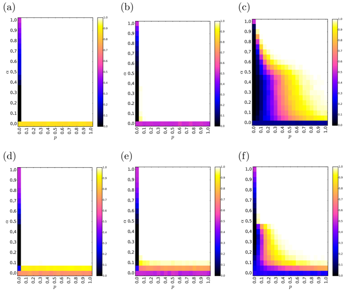
## Heatmap Series: Parameter Space Analysis (p vs. c) ### Overview The image displays a series of six heatmaps, labeled (a) through (f), arranged in a 2x3 grid. Each heatmap visualizes a scalar value (represented by color) as a function of two parameters, `p` and `c`, both ranging from 0.0 to 1.0. The plots appear to be from a scientific or technical study, likely exploring the behavior of a system, model, or function across a two-dimensional parameter space. The color scale is consistent across all plots, ranging from 0.0 (dark blue/purple) to 1.0 (bright yellow). ### Components/Axes * **Layout:** Six subplots in a 2x3 grid. Top row: (a), (b), (c). Bottom row: (d), (e), (f). * **Axes (for all subplots):** * **X-axis:** Labeled `p`. Ticks at 0.0, 0.1, 0.2, 0.3, 0.4, 0.5, 0.6, 0.7, 0.8, 0.9, 1.0. * **Y-axis:** Labeled `c`. Ticks at 0.0, 0.1, 0.2, 0.3, 0.4, 0.5, 0.6, 0.7, 0.8, 0.9, 1.0. * **Color Bar (Legend):** Positioned to the right of each subplot. It is a vertical gradient bar labeled with values from 0.0 at the bottom to 1.0 at the top, with intermediate ticks at 0.1 intervals. The color map transitions from dark blue/purple (low values, ~0.0) through magenta/pink to orange and finally bright yellow (high values, ~1.0). * **Text Language:** All labels, titles, and numbers are in English. ### Detailed Analysis **Subplot (a):** * **Trend:** High values (yellow) are concentrated exclusively along the very edges of the parameter space: where `p` is near 0.0 or `c` is near 0.0. The interior region (where both `p` and `c` are > ~0.05) is uniformly dark (value ~0.0). * **Data Points:** The highest values (1.0) appear as thin lines at `p=0.0` (for all `c`) and `c=0.0` (for all `p`). The transition from high to low is extremely sharp. **Subplot (b):** * **Trend:** Similar to (a), but the high-value region along the `c=0.0` axis is slightly broader and shows a gradient. The high-value line at `p=0.0` remains sharp. * **Data Points:** At `c=0.0`, values are high (yellow/orange) for `p` from 0.0 to ~0.1, then fade to low values. At `p=0.0`, values remain high for all `c`. **Subplot (c):** * **Trend:** This plot shows the most complex and extended gradient. High values originate from the corner `(p=0.0, c=0.0)` and spread diagonally outward. The region of high values forms a roughly triangular shape, with the gradient following a curve where `p` and `c` are both small. The value decreases smoothly as one moves away from the origin towards `(1.0, 1.0)`. * **Data Points:** The maximum (1.0) is at `(0,0)`. A broad region where `p + c < ~0.5` shows values > 0.5 (orange to yellow). The value at `(1.0, 1.0)` is very low (~0.0). **Subplot (d):** * **Trend:** Resembles a combination of (a) and (b). There is a sharp high-value line at `p=0.0`. Along `c=0.0`, there is a band of moderately high values that extends further into the `p` dimension than in (a) but is less extensive than in (c). * **Data Points:** High values at `p=0.0`. Along `c=0.0`, values are high (~0.8-0.9, orange) for `p` from 0.0 to ~0.2, then drop off. **Subplot (e):** * **Trend:** Very similar to (d), but the band of high values along `c=0.0` appears slightly narrower and the gradient slightly steeper. * **Data Points:** High values at `p=0.0`. Along `c=0.0`, the high-value region extends to `p` ~0.15 before dropping. **Subplot (f):** * **Trend:** Shows a distinct "L-shaped" or corner region of high values. The highest values are concentrated near the origin `(0,0)` and extend along both the `p=0.0` and `c=0.0` axes, but also fill a small square region where both parameters are small (e.g., `p<0.2, c<0.2`). The gradient is steep at the boundary of this region. * **Data Points:** The core high-value region (yellow) is roughly within `p<0.15` and `c<0.15`. Values drop sharply outside this square. The axes themselves remain high-value lines. ### Key Observations 1. **Common Feature:** All plots show that the output value is highest (1.0) when at least one parameter (`p` or `c`) is exactly 0.0. 2. **Progression of Complexity:** There is a clear progression from simple edge effects in (a) to a complex diagonal gradient in (c), and then to a confined corner region in (f). This suggests the six plots may represent different model variants, conditions, or time steps. 3. **Symmetry:** Plots (a), (d), and (e) are not symmetric with respect to the `p` and `c` axes; the effect of `p=0` is sharper than the effect of `c=0`. Plot (c) is more symmetric in its diagonal spread. Plot (f) shows symmetry within its corner region. 4. **Gradient Sharpness:** The transition from high to low values is sharpest in (a) and becomes more gradual in (c). Plots (d), (e), and (f) show intermediate sharpness. ### Interpretation These heatmaps likely visualize the output of a function `f(p, c)` where `p` and `c` are key parameters. The consistent maximum at the axes (`p=0` or `c=0`) suggests these parameter values represent a boundary condition, a default state, or a point of system failure/saturation where the output is maximized or fixed. * **Plot (a)** represents a scenario where the output is only non-zero at the absolute boundaries of the parameter space. This could indicate a system that is "off" or inactive except when at least one parameter is zero. * **Plot (c)** shows the most "well-behaved" or continuous response, where the output decays smoothly from a maximum at the origin. This is typical of many physical or statistical models where `(0,0)` is a natural origin point. * **Plots (b), (d), (e)** show intermediate behaviors, where the influence of one parameter (`c=0`) extends slightly into the space, creating a narrow band of activity. * **Plot (f)** suggests a system with a defined "active region" near the origin. Outside this small square of low `p` and `c` values, the output is minimal. This could model a system that only functions within a specific, limited parameter regime. The series as a whole demonstrates how changing an underlying condition (represented by the subplot label) dramatically alters the system's sensitivity to its parameters `p` and `c`. The progression from (a) to (c) might show the effect of increasing a coupling strength or relaxation time, while the progression from (d) to (f) might show the effect of a different type of constraint or nonlinearity. Without the accompanying figure caption or text, the exact meaning of `p`, `c`, and the difference between subplots remains speculative, but the visual data clearly maps out distinct response landscapes.