## Decision Tree Diagram: Admissible Tree for UCI Credit Data
### Overview
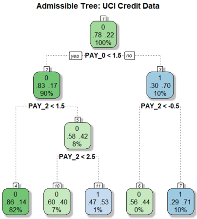
The image displays a binary decision tree model trained on the UCI Credit Card dataset. The tree is used to classify credit default risk. The structure is hierarchical, starting from a single root node and branching down to multiple leaf nodes based on specific feature thresholds. The primary color coding (green vs. blue) indicates the predicted class (0 for non-default, 1 for default) at each node.
### Components/Axes
* **Title:** "Admissible Tree: UCI Credit Data" (centered at the top).
* **Nodes:** Each node is a rounded rectangle containing four lines of text:
1. Node identifier number (top, in a small box).
2. Predicted class label (0 or 1).
3. Class distribution (two numbers, e.g., "78 22").
4. Percentage of total samples reaching that node.
* **Split Conditions:** Text labels on the connecting lines between nodes, specifying the feature and threshold used for the split (e.g., "PAY_0 < 1.5").
* **Branch Labels:** "yes" (left branch, condition true) and "no" (right branch, condition false).
* **Color Key (Implied):**
* **Green Nodes:** Predict class 0 (non-default).
* **Blue Nodes:** Predict class 1 (default).
* The intensity of the color appears to correlate with the confidence or purity of the node (darker for higher confidence).
### Detailed Analysis
**Tree Structure and Flow:**
The tree has a depth of 3 levels from the root.
1. **Root Node (Node 1):**
* **Position:** Top-center.
* **Data:** Class 0, Distribution: 78 (class 0) : 22 (class 1), 100% of samples.
* **Split:** `PAY_0 < 1.5`. This is the most important initial split.
2. **First-Level Children:**
* **Left Child (Node 2 - "yes" branch):**
* **Position:** Middle-left.
* **Data:** Class 0, Distribution: 83 : 17, 90% of samples.
* **Split:** `PAY_2 < 1.5`.
* **Right Child (Node 3 - "no" branch):**
* **Position:** Middle-right.
* **Data:** Class 1, Distribution: 30 : 70, 10% of samples.
* **Split:** `PAY_2 < -0.5`.
3. **Second-Level Children (Leaf Nodes from Node 2):**
* **Left Leaf (Node 4):**
* **Position:** Bottom-left.
* **Data:** Class 0, Distribution: 86 : 14, 82% of samples. **Leaf Node.**
* **Right Child (Node 5):**
* **Position:** Bottom-center-left.
* **Data:** Class 0, Distribution: 58 : 42, 8% of samples.
* **Split:** `PAY_2 < 2.5`.
4. **Third-Level Children (Leaf Nodes from Node 5):**
* **Left Leaf (Node 10):**
* **Position:** Bottom-center.
* **Data:** Class 0, Distribution: 60 : 40, 7% of samples. **Leaf Node.**
* **Right Leaf (Node 11):**
* **Position:** Bottom-center-right.
* **Data:** Class 1, Distribution: 47 : 53, 1% of samples. **Leaf Node.**
5. **Second-Level Children (Leaf Nodes from Node 3):**
* **Left Leaf (Node 6):**
* **Position:** Bottom-center-right.
* **Data:** Class 0, Distribution: 56 : 44, 0% of samples (likely a rounding of a very small percentage). **Leaf Node.**
* **Right Leaf (Node 7):**
* **Position:** Bottom-right.
* **Data:** Class 1, Distribution: 29 : 71, 10% of samples. **Leaf Node.**
**Feature Summary:**
The tree uses two features for splitting:
* `PAY_0`: Repayment status in September (the most recent month).
* `PAY_2`: Repayment status in July (two months prior).
### Key Observations
1. **Dominant Predictor:** The first split on `PAY_0 < 1.5` is highly effective. 90% of samples go left (likely "on-time" or "slight delay" payments), and only 10% go right (likely "significant delay" or default).
2. **Class Imbalance in Leaves:** The leaf nodes show varying levels of class purity. Node 4 is highly pure (86% class 0). Node 7 is strongly skewed towards class 1 (71%). Node 11 is nearly balanced (47% vs 53%).
3. **Sample Distribution:** The vast majority of samples (82%) end up in the most pure non-default leaf (Node 4). The high-risk leaf (Node 7) contains 10% of the total sample population.
4. **Feature Reuse:** The feature `PAY_2` is used for three different splits at different thresholds (1.5, -0.5, and 2.5), indicating its nuanced importance in refining the prediction after the initial `PAY_0` split.
### Interpretation
This decision tree provides a transparent, rule-based model for credit default prediction. The analysis suggests:
* **Primary Risk Factor:** A customer's most recent repayment status (`PAY_0`) is the strongest single indicator. A value below 1.5 (likely indicating payments are on time or only slightly late) places a customer in a much lower risk category.
* **Secondary Risk Refinement:** For customers with good recent payment history (`PAY_0 < 1.5`), their payment status from two months prior (`PAY_2`) is used to further stratify risk. A `PAY_2` value below 1.5 leads to the safest group (Node 4). Higher values of `PAY_2` indicate increasing risk, even if the most recent month is good.
* **High-Risk Profile:** Customers who fail the first check (`PAY_0 >= 1.5`) are already in a high-risk group (Node 3, 70% class 1). For them, `PAY_2` is used to identify an extreme risk subgroup: those with `PAY_2 >= -0.5` (Node 7) have a 71% default rate.
* **Model Behavior:** The tree prioritizes identifying safe customers (large, pure Node 4) while also creating specific rules to flag high-risk customers. The existence of a nearly balanced leaf (Node 11) indicates a segment where the model's prediction is less certain, based on the available features.
**In essence, the tree translates the complex credit data into a simple, auditable flowchart: "Check the latest payment status first. If good, check the status from two months ago to gauge consistency. If the latest status is bad, check the older status to identify the most severe cases."**