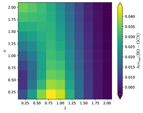
\n ## Heatmap: Acc_cost (BO-GCN) vs. λ and μ ### Overview This image is a 2D heatmap visualizing the relationship between two parameters, λ (lambda) on the x-axis and μ (mu) on the y-axis, and a performance metric labeled `Acc_cost (BO-GCN)`. The color intensity represents the value of this metric, with a color bar on the right providing the scale. The data suggests the performance of a system (likely a Bayesian Optimization - Graph Convolutional Network model) is highly sensitive to the combination of these two hyperparameters. ### Components/Axes * **Chart Type:** 2D Heatmap. * **X-Axis:** * **Label:** `λ` (Greek letter lambda). * **Scale & Ticks:** Linear scale from approximately 0.1 to 2.1. Major tick marks are present at 0.25, 0.50, 0.75, 1.00, 1.25, 1.50, 1.75, and 2.00. * **Y-Axis:** * **Label:** `μ` (Greek letter mu). * **Scale & Ticks:** Linear scale from approximately 0.1 to 2.1. Major tick marks are present at 0.25, 0.50, 0.75, 1.00, 1.25, 1.50, 1.75, and 2.00. * **Color Bar (Legend):** * **Position:** Vertically oriented on the right side of the heatmap. * **Label:** `Acc_cost (BO-GCN)`. This likely stands for "Accuracy Cost" or a similar performance metric for a BO-GCN model. * **Scale:** Continuous, ranging from a minimum of approximately **0.005** (dark purple) to a maximum of approximately **0.040** (bright yellow). * **Gradient:** The color gradient transitions from dark purple (lowest values) through blue, teal, and green to yellow (highest values). ### Detailed Analysis The heatmap displays a clear, non-uniform distribution of the `Acc_cost` metric across the λ-μ parameter space. * **Spatial Grounding & Trend Verification:** * **High-Value Region (Yellow/Green):** The highest values (bright yellow, ~0.040) are concentrated in a specific region. This region is located in the **bottom-left quadrant** of the heatmap, centered approximately at **λ ≈ 0.75 to 1.00** and **μ ≈ 0.25 to 0.50**. The color here is the brightest, indicating peak performance. * **Gradient Direction:** Moving away from this peak region, the values decrease. The gradient is not symmetric. * **Increasing λ (moving right):** There is a **sharp decline** in value. As λ increases beyond 1.00, the color rapidly shifts from green to teal to dark blue, even for low μ values. For λ > 1.50, the entire column is dark blue/purple regardless of μ. * **Increasing μ (moving up):** There is a **moderate decline** in value. As μ increases from 0.50 towards 2.00, the color shifts from yellow/green to teal and then to blue, especially for λ values less than 1.00. * **Low-Value Region (Dark Purple/Blue):** The lowest values (~0.005 - 0.010) are found in two primary areas: 1. The **top-right quadrant** (high λ > 1.50, high μ > 1.25). This area is uniformly dark purple. 2. The **far-right edge** (λ ≈ 2.00) across almost all μ values, which is a very dark blue/purple. * **Data Point Confirmation:** The brightest yellow cell aligns with the top of the color bar (~0.040). The darkest purple cells align with the bottom of the color bar (~0.005). ### Key Observations 1. **Optimal Parameter Zone:** There is a distinct "sweet spot" for the `Acc_cost` metric where λ is moderate (~0.75-1.00) and μ is low (~0.25-0.50). 2. **Asymmetric Sensitivity:** The metric is more sensitive to increases in λ than to increases in μ. A small increase in λ beyond 1.00 causes a more dramatic performance drop than a comparable increase in μ. 3. **Threshold Effect:** There appears to be a performance threshold around **λ = 1.00**. To the left of this line, values are generally higher (green/yellow). To the right, values drop significantly (blue/purple). 4. **Interaction Effect:** The parameters λ and μ interact. The negative effect of a high μ is exacerbated when λ is also high (top-right corner is the worst-performing region). Conversely, a low μ can partially buffer the negative effect of a moderately high λ. ### Interpretation This heatmap provides a visual guide for hyperparameter tuning of the BO-GCN model with respect to the `Acc_cost` metric. * **What the data suggests:** The model's performance (as measured by `Acc_cost`) is not linearly related to λ and μ. Instead, it exhibits a complex interaction with a clear optimum. The sharp decline past λ=1.00 suggests this parameter may control a regularization strength or a trade-off term where exceeding a critical value is detrimental. * **How elements relate:** λ and μ are likely coupled hyperparameters. The heatmap shows that optimizing one without considering the other is ineffective. The best performance requires a balanced, low-to-moderate setting for both, with a particular emphasis on keeping λ below 1.00. * **Notable Anomalies/Patterns:** The most striking pattern is the **cliff-like drop** in performance as λ crosses 1.00. This is a critical insight for anyone using this model, indicating that λ should be carefully constrained below this threshold. The relative stability of the metric for μ values below 0.75 (when λ is also low) suggests the model is more robust to changes in μ within that range. * **Practical Implication:** To achieve the best `Acc_cost`, one should set λ between 0.75 and 1.00 and μ between 0.25 and 0.50. Exploring parameter combinations outside this region, especially with λ > 1.25, is likely to yield poor results.