## Diagram: Algorithm Flowcharts
### Overview
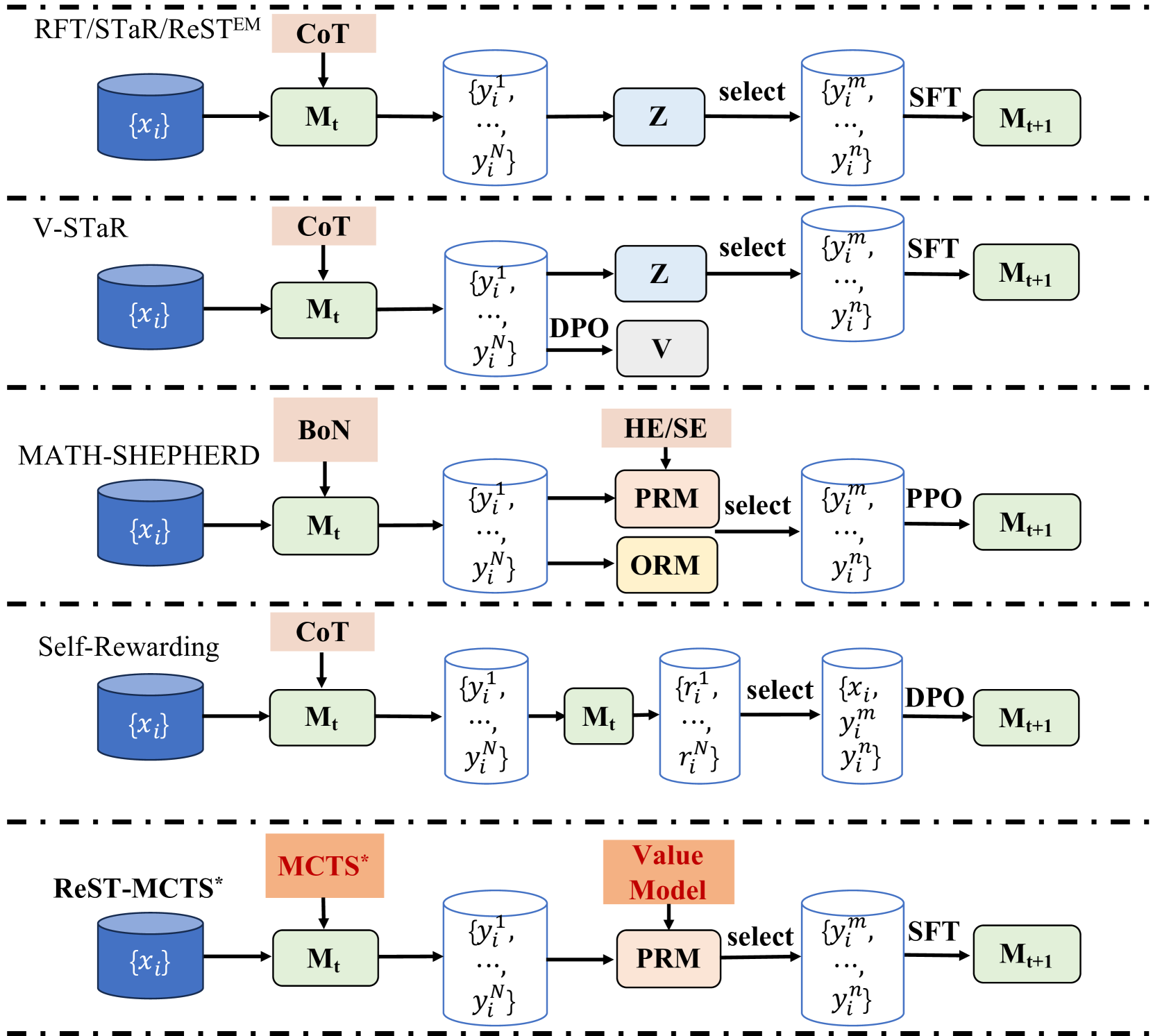
The image presents a series of flowcharts, each representing a different algorithm or method. The algorithms are RFT/STaR/ReST<sup>EM</sup>, V-STaR, MATH-SHEPHERD, Self-Rewarding, and ReST-MCTS*. Each flowchart illustrates the sequence of operations and data transformations within the respective algorithm.
### Components/Axes
Each flowchart consists of the following components:
- **Input Data:** Represented as a blue cylinder labeled "{x<sub>i</sub>}".
- **Model (M<sub>t</sub>):** Represented as a green rectangle.
- **Intermediate Data:** Represented as blue cylinders labeled with variations of "{y<sub>i</sub><sup>1</sup>, ..., y<sub>i</sub><sup>N</sup>}" or "{y<sub>i</sub><sup>m</sup>, ..., y<sub>i</sub><sup>n</sup>}".
- **Processing Steps:** Represented as light blue, light orange, or light red rectangles with labels such as "Z", "PRM", "ORM", "Value Model", "CoT", "BoN", "HE/SE", "DPO", "PPO", "SFT", "MCTS*".
- **Selection Steps:** Indicated by the word "select" and an arrow.
- **Output Data:** Represented as a green rectangle labeled "M<sub>t+1</sub>".
The flow direction is generally from left to right, indicating the sequence of operations.
### Detailed Analysis
**1. RFT/STaR/ReST<sup>EM</sup>**
- Input: {x<sub>i</sub>}
- Process: CoT (light red rectangle) -> M<sub>t</sub> (green rectangle)
- Intermediate Data: {y<sub>i</sub><sup>1</sup>, ..., y<sub>i</sub><sup>N</sup>}
- Process: Z (light blue rectangle) -> select {y<sub>i</sub><sup>m</sup>, ..., y<sub>i</sub><sup>n</sup>}
- Process: SFT (light green rectangle) -> M<sub>t+1</sub>
**2. V-STaR**
- Input: {x<sub>i</sub>}
- Process: CoT (light red rectangle) -> M<sub>t</sub> (green rectangle)
- Intermediate Data: {y<sub>i</sub><sup>1</sup>, ..., y<sub>i</sub><sup>N</sup>}
- Process: Z (light blue rectangle) -> select {y<sub>i</sub><sup>m</sup>, ..., y<sub>i</sub><sup>n</sup>}
- Process: DPO (light gray rectangle) and V (light gray rectangle)
- Process: SFT (light green rectangle) -> M<sub>t+1</sub>
**3. MATH-SHEPHERD**
- Input: {x<sub>i</sub>}
- Process: BoN (light red rectangle) -> M<sub>t</sub> (green rectangle)
- Intermediate Data: {y<sub>i</sub><sup>1</sup>, ..., y<sub>i</sub><sup>N</sup>}
- Process: HE/SE (light red rectangle) -> PRM (light orange rectangle) -> select {y<sub>i</sub><sup>m</sup>, ..., y<sub>i</sub><sup>n</sup>}
- Process: ORM (light yellow rectangle)
- Process: PPO (light green rectangle) -> M<sub>t+1</sub>
**4. Self-Rewarding**
- Input: {x<sub>i</sub>}
- Process: CoT (light red rectangle) -> M<sub>t</sub> (green rectangle)
- Intermediate Data: {y<sub>i</sub><sup>1</sup>, ..., y<sub>i</sub><sup>N</sup>}
- Process: M<sub>t</sub> (green rectangle)
- Intermediate Data: {r<sub>i</sub><sup>1</sup>, ..., r<sub>i</sub><sup>N</sup>}
- Process: select {x<sub>i</sub>, y<sub>i</sub><sup>m</sup>, ..., y<sub>i</sub><sup>n</sup>}
- Process: DPO (light gray rectangle) -> M<sub>t+1</sub>
**5. ReST-MCTS***
- Input: {x<sub>i</sub>}
- Process: MCTS* (light red rectangle) -> M<sub>t</sub> (green rectangle)
- Intermediate Data: {y<sub>i</sub><sup>1</sup>, ..., y<sub>i</sub><sup>N</sup>}
- Process: Value Model (light red rectangle) -> PRM (light orange rectangle) -> select {y<sub>i</sub><sup>m</sup>, ..., y<sub>i</sub><sup>n</sup>}
- Process: SFT (light green rectangle) -> M<sub>t+1</sub>
### Key Observations
- All algorithms start with input data {x<sub>i</sub>} and produce an output M<sub>t+1</sub>.
- The algorithms differ in their intermediate processing steps and data transformations.
- Several algorithms use "CoT" (Chain of Thought) as an initial processing step.
- "PRM" (likely Prompt Rewriting Module) appears in MATH-SHEPHERD and ReST-MCTS*.
- "DPO" (Direct Preference Optimization) appears in V-STaR and Self-Rewarding.
- "SFT" (Supervised Fine-Tuning) is a common final step before producing M<sub>t+1</sub>.
### Interpretation
The diagram illustrates the architectural differences between several reinforcement learning and language model training algorithms. The flowcharts highlight the key components and data flow within each algorithm, emphasizing the different strategies used for processing input data, generating intermediate representations, and optimizing the final model. The presence of common elements like "CoT" and "SFT" suggests shared underlying principles, while the unique processing steps indicate distinct approaches to problem-solving and model training. The diagram is useful for comparing and contrasting these algorithms at a high level.